This article describes best practices and techniques that every data analyst should know before bootstrapping in SAS.
The bootstrap method is a powerful statistical technique, but it can be a challenge to implement it efficiently.
An inefficient bootstrap program can take hours to run, whereas a well-written program can give you an answer in an instant.
If you prefer “instants” to “hours,” this article is for you! I’ve compiled dozens of resources that explain how to compute bootstrap statistics in SAS.

Overview: What is the bootstrap method?

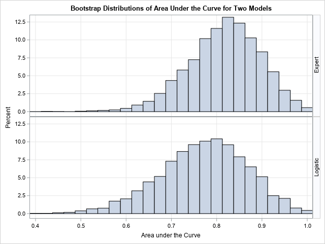
Recall that a bootstrap analysis enables you to investigate the sampling variability of a statistic without making any distributional assumptions about the population. For example, if you compute the skewness of a univariate sample, you get an estimate for the skewness of the population. You might want to know the range of skewness values that you might observe from a second sample (of the same size) from the population. If the range is large, the original estimate is imprecise. If the range is small, the original estimate is precise. Bootstrapping enables you to estimate the range by using only the observed data.

In general, the basic bootstrap method consists of four steps:

1. Compute a statistic for the original data.
2. Use the DATA step or PROC SURVEYSELECT to resample (with replacement) B times from the data. The resampling process should respect the null hypothesis or reflect the original sampling scheme. For efficiency, you should
   put all B random bootstrap samples into a single data set.
3. Use BY-group processing to compute the statistic of interest on each bootstrap sample. The BY-group approach is much faster than using macro loops.
   The union of the statistic is the bootstrap distribution, which approximates the sampling distribution of the statistic under the null hypothesis. Don’t forget to turn off ODS when you run BY-group processing!
4. Use the bootstrap distribution to obtain estimates for the bias and standard error of the statistic and confidence intervals for parameters.

The links in the previous list provide examples of best practices for bootstrapping in SAS. In particular, do not fall into the trap of using a macro loop to “resample, analyze, and append.” You will eventually get the correct bootstrap estimates, but you might wait a long time to get them!

The remainder of this article is organized by the three ways to perform bootstrapping in SAS:

• Programming: You can write a SAS DATA step program or a SAS/IML program that resamples from the data and analyzes each (re)sample. The programming approach gives you complete control over all aspects of the bootstrap analysis.
• Macros: You can use the %BOOT and %BOOTCI macros that are supplied by SAS. The macros handle a wide variety of common bootstrap analyses.
• Procedures: You can use bootstrap options that are built into several SAS procedures. The procedure internally implements the bootstrap method for a particular set of statistics.

Programming the basic bootstrap in SAS

The articles in this section describe how to program the bootstrap method in SAS for basic univariate analyses, for regression analyses, and for related resampling techniques such as the jackknife and permutation tests. This section also links to articles that describe how to generate bootstrap samples in SAS.

Examples of basic bootstrap analyses in SAS

• The basic bootstrap in SAS:
  SAS enables you to resample the data by using PROC SURVEYSELECT. When coupled with BY-group processing, you can perform a very efficient bootstrap analysis in SAS, including the estimate of standard errors and percentile-based confidence intervals.
• The basic bootstrap in SAS/IML: The SAS/IML language provides a compact language for bootstrapping, as shown in this basic bootstrap example.
• The smooth bootstrap: As originally conceived,
  a bootstrap sample contains replicates of the data. However, there are situations when “jittering” the data provides a better approximation of the sampling distribution.
• Bias-corrected and adjusted (BCa) confidence interval: For highly skewed data, the percentile-based confidence intervals are less efficient than the BCa confidence interval.
• Bootstrap the difference of means between two groups: This example shows how to bootstrap a statistic in a two-sample t test.
• Compute a p-value for a bootstrap analysis.
  

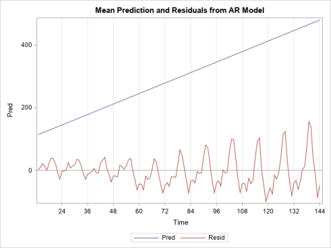
Examples of bootstrapping for regression statistics

When you bootstrap regression statistics, you have two choices for generating the bootstrap samples:

• Case resampling:
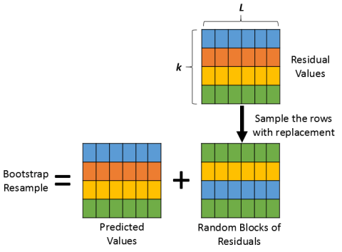
  You can resample the observations (cases) to obtain bootstrap samples of the responses and the explanatory variables.
• Residual resampling:
  Alternatively, you can bootstrap regression parameters by fitting a model and resampling from the residuals to obtain new responses.

Jackknife and permutation tests in SAS

• The jackknife method: The jackknife in an alternative nonparametric method for obtaining standard errors for statistics. It is deterministic because it uses leave-one-out samples rather than random samples.
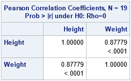
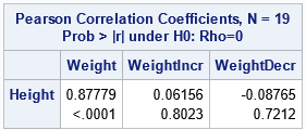
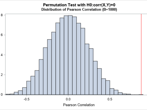
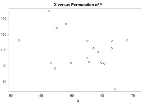
• Permutation tests: A
  permutation test is a resampling technique that is closely related to the bootstrap. You permute the observations between two groups to test whether the groups are significantly different.

Generate bootstrap sampling

An important part of a bootstrapping is generating multiple bootstrap samples from the data. In SAS, there are many ways to obtain the bootstrap samples:

• Sample with replacement: The most common resampling technique is to randomly sample with replacement from the data. You can use the SAS DATA step, the SURVEYSELECT procedure, or the SAMPLE function in SAS/IML.
• Samples in random order:
  It is sometimes useful to generate random samples in which the order of the observations is randomly permuted.
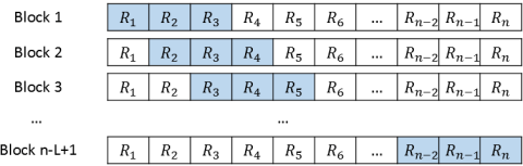
• Balanced bootstrap resampling:
  Instead of random samples, some experts advocate a resampling algorithm in which each observation appears exactly B times in the union of the B bootstrap samples.

Bootstrap macros in SAS

The SAS-supplied macros %BOOT, %JACK, and %BOOTCI,
can perform basic bootstrap analyses and jackknife analyses. However, they require a familiarity with writing and using SAS macros. If you are interested, I wrote an example that shows how to use the %BOOT and %BOOTCI macros for bootstrapping. The documentation also provides several examples.

SAS procedures that support bootstrapping

Many SAS procedures not only compute statistics but also provide standard errors or confidence intervals that enable you to infer whether an estimate is precise. Many confidence intervals are based on distributional assumptions about the population. (“If the errors are normally distributed, then….”) However, the following SAS procedures provide an easy way to obtain a distribution-free confidence interval by using the bootstrap. See the SAS/STAT documentation for the syntax for each procedure.

• PROC CAUSALMED introduced the BOOTSTRAP statement in SAS/STAT 14.3 (SAS 9.4M5). The statement enables you to compute bootstrap estimates of standard errors and confidence intervals for various effects and percentages of total effects.
• PROC MULTTEST supports the BOOTSTRAP and PERMUTATION options, which enable you to compute estimates of p-values that make no distributional assumptions.
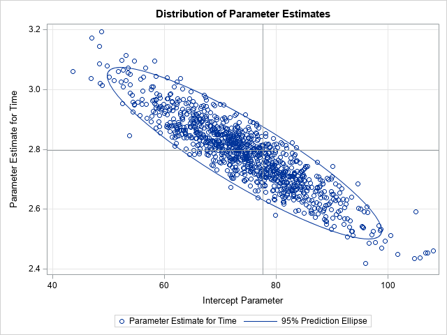
• PROC NLIN supports the BOOTSTRAP statement, which computes bootstrap confidence intervals for parameters and bootstrap estimates of the covariance of the parameter estimates.
• PROC QUANTREG supports the CI=RESAMPLING option to construct confidence intervals for regression quantiles.
• The SURVEYMEANS, SURVEYREG, SURVEYLOGISTIC, SURVEYPHREG, SURVEYIMPUTE and SURVEYFREQ procedures introduced the VARMETHOD=BOOTSTRAP option SAS 9.4M5. The option enables you to compute bootstrap estimates of variance.
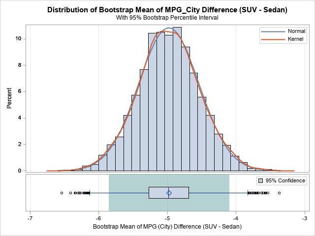
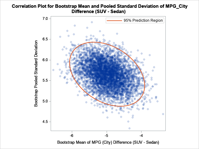
  With the exception of SURVEYIMPUTE, these procedures also support jackknife estimates. The jackknife is similar to the bootstrap but uses a leave-one-out deterministic scheme rather than random resampling.
• PROC TTEST introduced the BOOTSTRAP statement in SAS/STAT 14.3. The statement enables you to compute bootstrap standard error, bias estimates, and confidence limits for means and standard deviations in t tests. In SAS/STAT 15.1 (SAS 9.4M6), the TTEST procedure provides extensive graphics that visualize the bootstrap distribution.

Summary

Resampling techniques such as bootstrap methods and permutation tests are widely used by modern data analysts. But how you implement these techniques can make a huge difference between getting the results in a few seconds versus a few hours.
This article summarizes and consolidates many previous articles that demonstrate how to perform an efficient bootstrap analysis in SAS. Bootstrapping enable you to investigate the sampling variability of a statistic without making any distributional assumptions. In particular, the bootstrap is often used to estimate standard errors and confidence intervals for parameters.

Further Reading

• Cassell, David L. (2010) “BootstrapMania!: Re-Sampling the SAS Way”, Proceedings of
  the SAS Global Forum 2010 Conference.
• Vickery, John (2015) “Permit Me to Permute: A Basic Introduction to Permutation Tests”,
  Proceedings of
  the SAS Global Forum 2015 Conference.
• Wicklin, Rick (2013), “Resampling and Bootstrap Methods,” Chapter 15 in Simulating Data with SAS, SAS Institute Inc., Cary NC.

The post The essential guide to bootstrapping in SAS appeared first on The DO Loop.

When I run a bootstrap analysis, I create graphs to visualize the distribution of the bootstrap statistics. For example, in my article about how to bootstrap the difference of means in a two-sample t test, I included a histogram of the bootstrap distribution and added reference lines to indicate a confidence interval for the difference of means.

For t tests, the TTEST procedure supports the BOOTSTRAP statement, which automates the bootstrap process for standard one- and two-sample t tests. A new feature in SAS/STAT 15.1 (SAS 9.4M6) is that the TTEST procedure supports the PLOTS=BOOTSTRAP option, which automatically creates histograms, Q-Q plots, and scatter plots of various bootstrap distributions.

To demonstrate the new PLOTS=BOOTSTRAP option, I will use the same example that I used to demonstrate the BOOTSTRAP statement. The data are the sedans and SUVs in the Sashelp.Cars data. The research question is to estimate the difference in fuel efficiency, as measured by miles per gallon during city driving. The bootstrap analysis enables you to visualize the approximate sampling distribution of the difference-of-mean statistic and its standard deviation.
The following statements create the data and run PROC TTEST to generate the analysis. The PLOTS=BOOTSTRAP option generates the bootstrap graphs. The BOOTSTRAP statement request 5,000 bootstrap resamples and 95% confidence intervals, based on the percentiles of the bootstrap distribution:

/* create data set that has two categories: 'Sedan' and 'SUV' */
data Sample;
set Sashelp.Cars(keep=Type MPG_City);
if Type in ('Sedan' 'SUV');
run;
 
ods trace on;
title "Bootstrap Estimates with Percentile CI";
proc ttest data=Sample plots=bootstrap;
   class Type;
   var MPG_City;
   bootstrap / seed=123 nsamples=5000 bootci=percentile;
run;

The TTEST procedure creates seven tables and eight graphs.
The previous article displayed and discussed several tables, so here I display only two of the graphs.

The first graph is a histogram of the bootstrap distribution of the difference between the sample means for each vehicle type. The distribution appears to be symmetric and approximately normal. The middle of the distribution is close to -5, which is the point estimate for the difference in MPG_City between the SUVs and the sedans in the data. How much should we trust that point estimate? The green region indicates that 95% of the bootstrap samples had differences that were in the green area underneath the histogram, which is approximately [-5.9, -4.1]. This is a 95% confidence interval for the difference.

Similar histograms (not shown) are displayed for two other statistics: the pooled standard deviation (of the difference between means) and the Satterthwaite standard deviation. The procedure also creates Q-Q plots of the bootstrap distributions.

The second graph is a scatter plot that shows the joint bootstrap distribution of the mean difference and the pooled standard deviations of the difference, based on 5,000 bootstrap samples. You can see that the statistics are slightly correlated. A sample that has a large (absolute) mean difference also tends to have a relatively large standard deviation. The 95% prediction region for the joint distribution indicates how these two statistics co-vary among random samples.

In summary, the TTEST procedure in SAS/STAT 15.1 supports a new PLOTS=BOOTSTRAP option, which automatically creates many graphs that help you to visualize the bootstrap distributions of the statistics.
If you are conducting a bootstrap analysis for a t test, I highly recommend using the plots to visualize the bootstrap distributions and results

The post Graphs of bootstrap statistics in PROC TTEST appeared first on The DO Loop.

Many SAS procedures support the BY statement, which enables you to perform an analysis for subgroups of the data set. Although the SAS/IML language does not have a built-in “BY statement,” there are various techniques that enable you to perform a BY-group analysis. The two I use most often are the UNIQUE-LOC technique and the UNIQUEBY technique.
The first is more intuitive, the second is more efficient.
This article shows how to use SAS/IML to read and process BY-group data from a data set.

I previously showed that you can perform BY-group processing in SAS/IML by using the UNIQUEBY technique, so this article uses the UNIQUE-LOC technique.
The statistical application is simulating clusters of data. If you have a SAS data set that contains the centers and covariance matrices for several groups of observations, you can then read that information into SAS/IML and simulate new observations for each group by using a multivariate normal distribution.

Matrix operations and BY groups

A BY-group analysis in SAS/IML usually starts with a SAS data set that contains a bunch of covariance or correlation matrices.
A simple example is a correlation analysis of each species of flower in Fisher’s iris data set. The BY-group variable is the species of iris: Setosa, Versicolor, or Virginica. The variables are measurements (in mm) of the sepals and petals of 150 flowers, 50 from each species.
A panel of scatter plots for the iris data is shown to the right. You can see that the three species appear to be clustered. From the shapes of the clusters, you might decide to model each cluster by using a multivariate normal distribution.

You can use the OUTP= and COV options in PROC CORR to output mean and covariance statistics for each group, as follows:

proc corr data=sashelp.iris outp=CorrOut COV noprint;
   by Species;
   var Petal: Sepal:;
run;
 
proc print data=CorrOut(where=(_TYPE_ in ("N", "MEAN", "COV"))) noobs;
   where Species="Setosa";  /* just view information for one group */
   by Species  _Type_ notsorted;
   var _NAME_ Petal: Sepal:;
run;

The statistics for one of the groups (Species=’Setosa’) are shown. The number of observations in the group (N) is actually a scalar value, but it was replicated to fit into a rectangular data set.

Reading BY-group information into SAS/IML

This section reads the sample size, mean vector, and covariance matrix for all groups. A WHERE clause selects only the observations of interest:

/* Read in N, Mean, and Cov for each species. Use to create a parametric bootstrap 
   by simulating N[i] observations from a MVN(Mean[i], Cov[i]) distribution */
proc iml;
varNames = {'PetalLength' 'PetalWidth' 'SepalLength' 'SepalWidth'};
use CorrOut where (_TYPE_="N" & Species^=" ");       /* N */
read all var varNames into mN[rowname=Species];      /* read for all groups */
print mN[c=varNames];
 
use CorrOut where (_TYPE_="MEAN" & Species^=" ");    /* mean */
read all var varNames into mMean[rowname=Species];   /* read for all groups */
print mMean[c=varNames];
 
use CorrOut where (_TYPE_="COV" & Species^=" ");     /* covariance */
read all var varNames into mCov[rowname=Species];    /* read for all groups */
close;
print mCov[c=varNames];

The output (not shown) shows that the matrices mN, mMean, and mCov contain the vertical concatenation (for all groups) of the sample size, mean vectors, and covariance matrices, respectively.

The grouping variable is Species.
You can use the UNIQUE function to get the unique (sorted) values of the groups. You can then iterate over the unique values and use the LOC function to extract only the rows of the matrices that correspond to the ith group. What you do with that information depends on your application. In the following program, the information for each group is used to create a random sample from a multivariate normal distribution that has the same size, mean, and covariance as the ith group:

/* Goal: Write random MVN values in X to data set */
X = j(1, ncol(varNames), .);         /* X variables will be numeric */
Spec = BlankStr(nleng(Species));     /* and Spec will be character */
create SimOut from X[rowname=Spec colname=varNames]; /* open for writing */
 
/* The BY-group variable is Species */
call randseed(12345);
u = unique(Species);                 /* get unique values for groups */
do i = 1 to ncol(u);                 /* iterate over unique values */
   idx = loc(Species=u[i]);          /* rows for the i_th group */
   N = mN[i, 1];                     /* extract scalar from i_th group */
   mu = mMean[i,];                   /* extract vector from i_th group */
   Sigma = mCov[idx,];               /* extract matrix from i_th group */
   /* The parameters for this group are now in N, mu, and Sigma.
      Do something with these values. */
   X = RandNormal(N, mu, Sigma);     /* simulate obs for the i_th group */
   X = round(X);                     /* measure to nearest mm */
   Spec = j(N, 1, u[i]);             /* ID for this sample */
   append from X[rowname=Spec];
end;
close SimOut;
quit;
 
ods graphics / attrpriority=none;
title "Parametric Bootstrap Simulation of Iris Data"; 
proc sgscatter data=SimOut(rename=(Spec=Species));
   matrix Petal: Sepal: / group=Species;
run;

The simulation has generated a
new set of clustered data. If you compare the simulated data with the original, you will notice many statistical similarities.

Although the main purpose of this article is to discuss BY-group processing in SAS/IML, I want to point out that the simulation in this article is an example of the parametric bootstrap.
Simulating Data with SAS (Wicklin, 2013) states that “the parametric bootstrap is nothing more than the process of fitting a model
distribution to the data and simulating data from the fitted model.” That is what happens in this program. The sample means and covariance matrices are used as parameters to generate new synthetic observations. Thus, the parametric bootstrap technique is really a form of simulation where the parameters for the simulation are obtained from the data.

In conclusion, sometimes you have many matrices in a SAS data set, each identified by a categorical variable. You can perform “BY-group processing” in SAS/IML by reading in all the matrices into a big matrix and then use the UNIQUE-LOC technique to iterate over each matrix.

The post Matrix operations and BY groups appeared first on The DO Loop.

At SAS Global Forum 2019, Daymond Ling presented an interesting discussion of binary classifiers in the financial industry. The discussion is motivated by a practical question: If you deploy a predictive model, how can you assess whether the model is no longer working well and needs to be replaced?

Daymond discussed the following three criteria for choosing a model:

1. Discrimination: The ability of the binary classifier to predict the class of a labeled observation. The area under an ROC curve is one measure of a binary model’s discrimination power. In SAS, you can compute the ROC curve for any predictive model.
2. Accuracy: The ability of the model to estimate the probability of an event. The calibration curve is a graphical indication of a model’s accuracy. In SAS, you can compute a calibration curve manually, or you can use PROC LOGISTIC in SAS/STAT 15.1 to automatically compute a calibration curve.
3. Stability: Point estimates are often used to choose a model, but you should be aware of the variability of the estimates. This is a basic concept in statistics: When choosing between two unbiased estimators, you should usually choose the one that has smaller variance. SAS procedures provide (asymptotic) standard errors for many statistics such as the area under an ROC curve. If you have reason to doubt the accuracy of an asymptotic estimate, you can use bootstrap methods in SAS to estimate the sampling distribution of the statistic.

Estimates of model stability

My article about comparing the ROC curves for predictive models contains two competing models: A model from using PROC LOGISTIC and an “Expert model” that was constructed by asking domain experts for their opinions. (The source of the models is irrelevant; you can use any binary classifier.)
You can download the SAS program that produces the following table, which estimates the area under each ROC curve, the standard error, and 90% confidence intervals:

The “Expert” model has a larger Area statistic and a smaller standard error, so you might choose to deploy it as a “champion model.”

In his presentation, Daymond asked an important question. Suppose one month later you run the model on a new batch of labeled data and discover that the area under the ROC curve for the new data is only 0.73. Should you be concerned? Does this indicate that the model has degraded and is no longer suitable? Should you cast out this model, re-train all the models (at considerable time and expense), and deploy a new “champion”?

The answer depends on whether you think Area = 0.73 represents a degraded model or whether it can be attributed to sampling variability. The statistic 0.73 is barely more than 1 standard error away from the point estimate, and you will recall that 68% of a normal distribution is within one standard deviation of the mean. From that point of view, the value 0.73 is not surprising. Furthermore, the 90% confidence interval indicates that if you run this model every day for 100 days, you will probably encounter statistics lower than 0.68 merely due to sampling variability. In other words, a solitary low score might not indicate that the model is no longer valid.

Bootstrap estimates of model stability

If “asymptotic normality” makes you nervous, you can use the bootstrap method to obtain estimates of the standard error and the distribution of the Area statistic. The following table summarizes the results of 5,000 bootstrap replications.
The results are very close to the asymptotic results in the previous table.
In particular, the standard error of the Area statistic is estimated as 0.08 and in 90% of the bootstrap samples, the Area was in the interval [0.676, 0.983]. The conclusion from the bootstrap computation is the same as for the asymptotic estimates: you should expect the Area statistic to bounce around. A value such as 0.73 is not unusual and does not necessarily indicate that the model has degraded.

You can use the bootstrap computations to graphically reveal the stability of the two models. The following comparative histogram shows the bootstrap distributions of the Area statistic for the “Expert” and “Logistic” models. You can see that not only is the upper distribution shifted to the right, but it has less variance and therefore greater stability.

I think Daymond’s main points are important to remember. Namely, discrimination and accuracy are important for choosing a model, but understanding the stability of the model (the variation of the estimates) is essential for determining when a model is no longer working well and should be replaced. There is no need to replace a model for a “bad score” if that score is within the range of typical statistical variation.

References

Ling, D. (2019), “Measuring Model Stability”, Proceedings of the SAS Global Forum 2019 Conference.

Download the complete SAS program that creates the analyses and graphs in this article.

The post Discrimination, accuracy, and stability in binary classifiers appeared first on The DO Loop.

I recently read an article that describes ways to compute confidence intervals for the difference in a percentile between two groups. In Eaton, Moore, and MacKenzie (2019), the authors describe a problem in hydrology. The data are the sizes of pebbles (grains) in rivers at two different sites. The authors ask whether the p_th percentile of size is significantly different between the two sites. They also want a confidence interval for the difference. The median (50th percentile) and 84th percentile were the main focus of their paper.

For those of us who are not hydrologists, consider a sample from group ‘A’ and a sample from group ‘B’. The problem is to test whether the p_th percentile is different in the two groups and to construct a confidence interval for the difference.

The authors show two methods: a binomial-based probability model (Section 2) and a bootstrap confidence interval (Section 3). However,
there is another option: use quantile regression to estimate the difference in the quantiles and to construct a confidence interval.
In this article, I show the computation for the 50th and 84th percentiles and compare the results to a bootstrap estimate.
You can download the SAS program that creates the analyses and graphs in this article.

If you are not familiar with quantile regression, see my previous article about how to use quantile regression to estimate the difference between two medians.

A data distribution of particle sizes

For convenience, I simulated samples for the sizes of pebbles in two stream beds:

• For Site ‘A’, the sizes are lognormally distributed with μ=0.64 and σ=1.
  For the LN(0.64, 1) distribution, the median pebble size is 1.9 mm and the size for the 84th percentile is 5.1 mm.
• For Site ‘B’, the sizes are lognormally distributed with μ=0.53 and σ=1.
  For the LN(0.53, 1) distribution, the median pebble size is 1.7 mm and the size for the 84th percentile is 4.6 mm.

I assume that sizes are measured to the nearest 0.1 mm.
I simulated 500 pebbles from Site ‘A’ and 300 pebbles from Site ‘B’.
You can use PROC UNIVARIATE in SAS to compute a comparative histogram and to compute the percentiles. The sample distributions are shown below:

For Site ‘A’, the estimates for the sample median and 84th percentile are 2.05 mm and 5.1 mm, respectively.
For Site ‘B’, the estimates are 1.60 mm and 4.7 mm, respectively. These estimates are close to their respective parameter values.

Estimate difference in percentiles

The QUANTREG procedure in SAS makes it easy to estimate the difference in the 50th and 84th percentiles between the two groups. The syntax for the QUANTREG procedure is similar to other SAS regression procedures such as PROC GLM:

proc quantreg data=Grains;
   class Site;
   model Diameter = Site / quantile=0.5 0.84;
   estimate 'Diff in Pctl' Site 1 -1 / CL;
run;

The output from PROC QUANTREG shows estimates for the difference between the percentiles of the two groups.
For the 50th percentile, an estimate for the difference is 0.4 with a 95% confidence of [0.09, 0.71].
Because 0 is not in the confidence interval, you can conclude that the median pebble size at Site ‘A’ is significantly different from the median pebble size at Site ‘B’.
For the 84th percentile, an estimate for the difference is 0.3 with a 95% confidence of [-0.57, 1.17].
Because 0 is in the interval, the difference between the 84th percentiles is not significantly different from 0.

Methods for estimating confidence intervals

The QUANTREG procedure supports several different methods for estimating a confidence interval:
sparsity, rank, and resampling.
The estimates in the previous section are by using the RANK method, which is the default for smaller data sets. You can use the CI= option on the PROC QUANTREG statement to use these methods and to specify options for the methods. The following graph summarizes the results for four combinations of methods and options. The results of the analysis do not change: The medians are significantly different but the 84th percentiles are not.

A comparison with bootstrap estimates

When you use a resampling-based estimate for the confidence interval, the interval depends on the random number seed, the algorithm used to generate random numbers, and the number of bootstrap iterations. This can make it hard to compare Monte Carlo results to the results from deterministic statistical methods. Nevertheless, I will present one result from a bootstrap analysis of the simulated data. The following table shows the bootstrap percentile estimates (used by Eaton, Moore, and MacKenzie (2019)) for the difference between percentiles.

The confidence intervals (the Lower and Upper columns of the table) are comparable to the intervals produced by PROC QUANTREG. The confidence interval for the difference between medians seems equivalent. The bootstrap interval for the 84th percentile is shifted to the right relative to the QUANTREG intervals. However, the inferences are the same: the medians are different but there is no significant difference between the 84th percentiles.

The following histogram shows the difference between the 84th percentiles for 5,000 bootstrap samples.
The confidence interval is determined by the 2.5th and 97.5th percentiles of the bootstrap distribution.
The computation requires only a short SAS/IML program, which runs very quickly.

Summary

Data analysts might struggle to find an easy way to compute the difference between percentiles for two (or more) groups. A recent paper by Eaton, Moore, and MacKenzie (2019) proposes one solution, which is to use resampling methods.
An alternative is to use quantile regression to estimate the difference between percentiles, as shown in this article. I demonstrate the method by using simulated data of the form studied by Eaton, Moore, and MacKenzie.

You can download the SAS program that creates the analyses and graphs in this article.

The post How to estimate the difference between percentiles appeared first on The DO Loop.

A fundamental principle of data analysis is that a statistic is an estimate of a parameter for the population. A statistic is calculated from a random sample. This leads to uncertainty in the estimate: a different random sample would have produced a different statistic.
To quantify the uncertainty, SAS procedures often support options that estimate standard errors for statistics and confidence intervals for parameters.

Of course, if statistics have uncertainty, so, too, do functions of the statistics. For complicated functions of the statistics,
the bootstrap method might be the only viable technique for quantifying the uncertainty.

This article shows how to obtain confidence intervals for the eigenvalues of a correlation matrix.
The eigenvalues are complicated functions of the correlation estimates.
The eigenvalues are used in a principal component analysis (PCA) to decide how many components to keep in a dimensionality reduction.
There are two main methods to estimate confidence intervals for eigenvalues: an asymptotic (large sample) method, which assumes that the eigenvalues are multivariate normal, and a bootstrap method, which makes minimal distributional assumptions.

The following sections show how to compute each method.
A graph of the results is shown to the right. For the data in this article, the bootstrap method generates confidence intervals that are more accurate than the asymptotic method.

This article was inspired by
Larsen and Warne (2010), “Estimating confidence intervals for
eigenvalues in exploratory factor analysis.” Larsen and Warne discuss why confidence intervals can be useful when deciding how many principal components to keep.

Eigenvalues in principal component analysis

To demonstrate the techniques, let’s perform a principal component analysis (PCA) on the four continuous variables in the Fisher Iris data. In SAS, you can use PROC PRINCOMP to perform a PCA, as follows:

%let DSName = Sashelp.Iris;
%let VarList = SepalLength SepalWidth PetalLength PetalWidth;
 
/* 1. compute value of the statistic on original data */
proc princomp data=&DSName STD plots=none;     /* stdize PC scores to unit variance */
   var &VarList;
   ods select ScreePlot Eigenvalues NObsNVar;
   ods output Eigenvalues=EV0 NObsNVar=NObs(where=(Description="Observations"));
run;
 
proc sql noprint;                              
 select nValue1 into :N from NObs;   /* put the number of obs into macro variable, N */
quit;
%put &=N;

The first table shows that there are 150 observations. The second table displays the eigenvalues for the sample, which are 2.9, 0.9, 0.15, and 0.02.
If you want a graph of the eigenvalues, you can use the PLOTS(ONLY)=SCREE option on the PROC PRINCOMP statement.
The ODS output statement creates SAS data set from the tables.
The PROC SQL call creates a macro variable, N, that contains the number of observations.

Asymptotic confidence intervals

If a sample size, n, is large enough, the sampling distribution of the eigenvalues is approximately multivariate normal (Larsen and Ware (2010, p. 873)). If g is an eigenvalue for a correlation matrix, then an asymptotic confidence interval is
     g ± z^* sqrt( 2 g² / n )
where z^* is the standard normal quantile, as computed in the following program:

/* Asymptotic CIs for eigenvalues (Larsen and Warne (2010, p. 873) */
data AsympCI;
set EV0;
alpha = 0.05;
z = quantile("Normal", 1 - alpha/2);  /* = 1.96 */
SE = sqrt(2*Eigenvalue**2 / &N);
Normal_LCL = Eigenvalue - SE;         /* g +/- z* sqrt(2 g^2 / n) */
Normal_UCL = Eigenvalue + SE;
drop alpha z SE;
run;
 
proc print data=AsympCI noobs;
   var Number Eigenvalue Normal_LCL Normal_UCL;
run;

The lower and upper confidence limits are shown for each eigenvalue.
The advantage of this method is its simplicity.
The intervals assume that the distribution of the eigenvalues is multivariate normal, which will occur when the sample size is very large. Since N=150 does not seem “very large,” it is not clear whether these confidence intervals are valid. Therefore, let’s estimate the confidence intervals by using the bootstrap method and compare the bootstrap intervals to the asymptotic intervals.

Bootstrap confidence intervals for eigenvalues

The bootstrap computations in this section follow the strategy outlined in the article “Compute a bootstrap confidence interval in SAS.” (For additional bootstrap tips, see “The essential guide to bootstrapping in SAS.”) The main steps are:

1. Compute a statistic for the original data. This was done in the previous section.
2. Use PROC SURVEYSELECT to resample (with replacement) B times from the data. For efficiency,
   put all B random bootstrap samples into a single data set.
3. Use BY-group processing to compute the statistic of interest on each bootstrap sample.
   The union of the statistics is the bootstrap distribution, which approximates the sampling distribution of the statistic. Remember to turn off ODS when you run BY-group processing!
4. Use the bootstrap distribution to obtain confidence intervals for the parameters.

The steps are implemented in the following SAS program:

/* 2. Generate many bootstrap samples */
%let NumSamples = 5000;       /* number of bootstrap resamples */
proc surveyselect data=&DSName NOPRINT seed=12345
     out=BootSamp(rename=(Replicate=SampleID))
     method=urs              /* resample with replacement */
     samprate=1              /* each bootstrap sample has N observations */
     /* OUTHITS                 option to suppress the frequency var */
     reps=&NumSamples;       /* generate NumSamples bootstrap resamples */
run;
 
/* 3. Compute the statistic for each bootstrap sample */
/* Suppress output during this step:
   https://blogs.sas.com/content/iml/2013/05/24/turn-off-ods-for-simulations.html
*/
%macro ODSOff();   ods graphics off; ods exclude all;  ods noresults;   %mend;
%macro ODSOn();    ods graphics on;  ods exclude none; ods results;     %mend;
 
%ODSOff;
proc princomp data=BootSamp STD plots=none;
   by SampleID;
   freq NumberHits;
   var &VarList;
   ods output Eigenvalues=EV(keep=SampleID Number Eigenvalue);
run;
%ODSOn;
 
/* 4. Estimate 95% confidence interval as the 2.5th through 97.5th percentiles of boostrap distribution */
proc univariate data=EV noprint;
   class Number;
   var EigenValue;
   output out=BootCI pctlpre=Boot_ pctlpts=2.5  97.5  pctlname=LCL UCL;
run;
 
/* merge the bootstrap CIs with the normal CIs for comparison */
data AllCI;
   merge AsympCI(keep=Number Eigenvalue Normal:) BootCI(keep=Number Boot:);
   by Number;
run;
 
proc print data=AllCI noobs;
   format Eigenvalue Normal: Boot: 5.3;
run;

The table displays the bootstrap confidence intervals (columns 5 and 6) next to the asymptotic confidence intervals (columns 3 and 4).
It is easier to compare the intervals if you visualize them graphically, as follows:

/* convert from wide to long */
data CIPlot;
   set AllCI;
   Method = "Normal   "; LCL = Normal_LCL; UCL = Normal_UCL; output;
   Method = "Bootstrap"; LCL = Boot_LCL; UCL = Boot_UCL; output;
   keep Method Eigenvalue Number LCL UCL;
run;
 
title "Comparison of Normal and Bootstrap Confidence Intervals";
title2 "Eigenvalues of the Correlation Matrix for the Iris Data";
ods graphics / width=480px height=360px;
proc sgplot data=CIPlot;
   scatter x=Eigenvalue y=Number / group=Method clusterwidth=0.4
           xerrorlower=LCL xerrorupper=UCL groupdisplay=cluster;
   yaxis grid type=discrete colorbands=even colorbandsattrs=(color=gray transparency=0.9);
   xaxis grid;
run;

The graph is shown at the top of this article. The graph nicely summarizes the comparison. For the first (largest) eigenvalue, the bootstrap confidence interval is about half as wide as the normal confidence interval. Thus, the asymptotic result seems too wide for these data. For the other eigenvalues, the normal confidence intervals appear to be too narrow.

If you graph the bootstrap distribution, you can see that the bootstrap distribution does not appear to be multivariate normal. This presumably explains why the asymptotic intervals are so different from the bootstrap intervals. For completeness, the following graph shows a matrix of scatter plots and marginal histograms for the bootstrap distribution. The histograms indicate skewness in the bootstrap distribution.

Summary

This article shows how to compute confidence intervals for the eigenvalues of an estimated correlation matrix.
The first method uses a formula that is valid when the sampling distribution of the eigenvalues is multivariate normal. The second method uses bootstrapping to approximate the distribution of the eigenvalues, then uses percentiles of the distribution to estimate the confidence intervals. For the Iris data, the bootstrap confidence intervals are substantially different from the asymptotic formula.

The post Confidence intervals for eigenvalues of a correlation matrix appeared first on The DO Loop.

For ordinary least squares (OLS) regression, you can use a basic bootstrap of the residuals (called residual resampling) to perform a bootstrap analysis of the parameter estimates. This is possible because an assumption of OLS regression is that the residuals are independent. Therefore, you can reshuffle the residuals to get each bootstrap sample.

For a time series, the residuals are not independent. Rather, if you fit a model to the data, the residuals at time t+i are often close to the residual at time t for small values of i. This is known as autocorrelation in the error component.
Accordingly, if you want to bootstrap the residuals of a time series, it is not correct to randomly shuffle the residuals, which would destroy the autocorrelation. Instead, you need to randomly choose a block of residuals (for example, at times t, t+1, …, and t+L) and use those blocks of residuals to create bootstrap resamples. You repeatedly choose random blocks until you have enough residuals to create a bootstrap resample.

There are several ways to choose blocks:

• The simplest way is to choose from non-overlapping blocks of a fixed length, L. This is called the simple block bootstrap
  and is described in this article.
• Only slightly more complicated is to allow the blocks of length L to overlap. This is called the moving block bootstrap
  and is described in a separate article.
• A more complicated scheme (but which has superior statistical properties) is to allow the length of the blocks to vary. This is called the stationary block bootstrap
  and is described in a third article.

Create the residuals

There are many ways to fit a model to a time series and to obtain the model residuals. Trovero and Leonard (2018) discuss several modern methods to fit trends, cycles, and seasonality by using SAS 9.4 or SAS Viya. To get the residuals, you will want to fit an additive model. In this article, I will use the Sashelp.Air data and will fit a simple additive model (trend plus noise) by using the AUTOREG procedure in SAS/ETS software.

The Sashelp.Air data set has 144 months of data. The following SAS DATA step drops the first year of data, which leaves 11 years of 12 months. I am doing this because I am going to use blocks of size L=12, and I think the example will be clearer if there are 11 blocks of size 12 (rather than 12 blocks).

data Air;
set Sashelp.Air;
if Date >= '01JAN1950'd;   /* exclude first year of data */
Time = _N_;                /* the observation number */
run;
 
title "Original Series: Air Travel";
proc sgplot data=Air;
   series x=Time y=Air;
   xaxis grid; yaxis grid;
run;

The graph suggests that the time series has a linear trend. The following call to PROC AUTOREG fits a linear model to the data. The predicted mean and residuals are output to the OutReg data set as the PRED and RESID variables, respectively. The call to PROC SGPLOT overlays a graph of the trend and a graph of the residuals.

/* Similar to Getting Started example in PROC AUTOREG */
proc autoreg data=Air plots=none outest=RegEst;
   AR12: model Air = Time / nlag=12;
   output out=OutReg pm=Pred rm=Resid;  /* mean prediction and residuals */
   ods select FinalModel.ParameterEstimates ARParameterEstimates;
run;
 
title "Mean Prediction and Residuals from AR Model";
proc sgplot data=OutReg;
   series x=Time y=Pred;
   series x=Time y=Resid;
   refline 0 / axis=y;
   xaxis values=(24 to 144 by 12) grid valueshint;
run;

The parameter estimates are shown for the linear model. On average, airlines carried an additional 2.8 thousand passengers per month during this time period.
The graph shows the decomposition of the series into a linear trend and residuals. I added vertical lines to indicate the blocks of residuals that are used in the next section.
The first block contains the residuals for times 13-24. The second block contains the residuals for times 25-36, and so forth until the 11th block, which contains the residuals for times 133-144.

Set up the simple block bootstrap

For the simple bootstrap, the length of the blocks (L) must evenly divide the length of the series (n), which means that k = n / L is an integer.
Because I dropped the first year of observations from Sashelp.Air, there are n=132 observations. I will choose the block size to be L=12, which means that there are k=11 non-overlapping blocks.

Each bootstrap resample is formed by randomly choosing k blocks (with replacement) and add those residuals to the predicted values.
Think about putting the n predicted values and residuals into a matrix in row-wise order. The first L observations are in the first row, the next L are in the second row, and so forth. Thus, the matrix has k rows and L columns.
The original series is of the form Predicted + Residuals, where the plus sign represents matrix addition.
For the simple block bootstrap, each bootstrap resample is obtained by resampling the rows of the residual array and adding the rows together to obtain a new series of the form Predicted + (Random Residuals). This process is shown schematically in the following figure.

You can use the SAS/IML language to implement the simple block bootstrap. The following call to PROC IML reads in the original predicted and residual values and reshapes then vectors into k x L matrices (P and R, respectively). The SAMPLE function generates a sample (with replacement) of the vector 1:k, which is used to randomly select rows of the R matrix. To make sure that the process is working as expected, you can create one bootstrap resample and graph it. It should resemble the original series:

/* SIMPLE BLOCK BOOTSTRAP */
%let L = 12;
proc iml;
call randseed(12345);
/* the original series is Y = Pred + Resid */
use OutReg;
   read all var {'Time' 'Pred' 'Resid'};
close;
 
/* For the Simple Block Bootstrap, the length of the series (n) 
   must be divisible by the block length (L). */
n = nrow(Pred);          /* length of series */
L = &L;                  /* length of each block */
k = n / L;               /* number of non-overlapping blocks */
if k ^= int(k) then 
   ABORT "The series length is not divisible by the block length";
 
/* Trick: reshape data into k x L matrix. Each row is block of length L */
P = shape(Pred, k, L);
R = shape(Resid, k, L); /* non-overlapping residuals (also k x L) */
 
/* Example: Generate one bootstrap resample by randomly selecting from the residual blocks */
idx = sample(1:nrow(R), k);     /* sample (w/ replacement) of size k from the set 1:k */
YBoot = P + R[idx,];
title "One Bootstrap Resample";
title2 "Simple Block Bootstrap";
refs = "refline " + char(do(12,nrow(Pred),12)) + " / axis=x;";
call series(Time, YBoot) other=refs;

The graph shows one bootstrap resample. The residuals from arbitrary blocks are concatenated until there are n residuals. These are added to the predicted value to create a “new” series, which is a bootstrap resample. You can generate a large number of bootstrap resamples and use them to perform inferences for time series statistics.

Implement the simple block bootstrap in SAS

You can repeat the process in a loop to generate more resamples. The following statements generate B=1000 bootstrap resamples.
These are written to a SAS data set (BootOut). The program uses a technique in which the results of each computation are immediately written to a SAS data set, which is very efficient. The program writes the Time variable, the resampled series (YBoot), and an ID variable that identifies each bootstrap sample.

/* The simple block bootstrap repeats this process B times
   and usually writes the resamples to a SAS data set. */
B = 1000;
J = nrow(R);              /* J=k for non-overlapping blocks, but prepare for moving blocks */
SampleID = j(n,1,.);
create BootOut var {'SampleID' 'Time' 'YBoot'};  /* open data set outside of loop */
do i = 1 to B;
   SampleId[,] = i;       /* fill array: https://blogs.sas.com/content/iml/2013/02/18/empty-subscript.html */
   idx = sample(1:J, k);  /* sample of size k from the set 1:k */
   YBoot = P + R[idx,];
   append;                /* append each bootstrap sample */
end;
close BootOut;
QUIT;

The BootOut data set contains B=1000 bootstrap samples. You can efficiently analyze the samples by using a BY statement. For example, suppose that you want to investigate how the parameter estimates for the trend line vary among the bootstrap samples. You can run PROC AUTOREG on each bootstrap sample by using BY-group processing. Be sure to suppress ODS output during the BY-group analysis, and write the desired statistics to an output data set (BootEst), as follows:

/* Analyze the bootstrap samples by using a BY statement. See
   https://blogs.sas.com/content/iml/2012/07/18/simulation-in-sas-the-slow-way-or-the-by-way.html
*/
proc autoreg data=BootOut plots=none outest=BootEst noprint;
   by SampleID;
   AR12: model YBoot = Time / nlag=12;
run;
 
/* OPTIONAL: Use PROC MEANS or PROC UNIVARIATE to estimate standard errors and CIs */
proc means data=BootEst mean stddev P5 P95;
   var Intercept Time _A:;
run;
 
title "Distribution of Parameter Estimates";
proc sgplot data=BootEst;
   scatter x=Intercept y=Time;
   xaxis grid; yaxis grid; 
   refline 77.5402 / axis=x;
   refline 2.7956  / axis=y;
run;

The scatter plot shows the bootstrap distribution of the parameter estimates of the linear trend. The reference lines indicate the parameter estimates for the original data. You can use the bootstrap distribution for inferential statistics such as estimation of standard errors, confidence intervals, the covariance of estimates, and more.

You can perform a similar bootstrap analysis for any other statistic that is generated by any time series analysis. The important thing is that the block bootstrap is performed on some sort of residual or “noise” component, so be sure to remove the trend, seasonality, cycles, and so forth and then bootstrap the remainder.

Summary

This article shows how to perform a simple block bootstrap on a time series in SAS. First, you need to decompose the series into additive components: Y = Predicted + Residuals. You then choose a block length (L), which (for the simple block bootstrap) must divide the total length of the series (n). Each bootstrap resample is generated by randomly choosing blocks of residuals and adding them to the predicted model. This article uses the SAS/IML language to perform the simple block bootstrap in SAS.

In practice, the simple block bootstrap is rarely used. However, it illustrates the basic ideas for bootstrapping a time series, and it provides a foundation for more sophisticated bootstrap methods.

The post The simple block bootstrap for time series in SAS appeared first on The DO Loop.

As I discussed in a previous article, the simple block bootstrap is a way to perform a bootstrap analysis on a time series. The first step is to decompose the series into additive components: Y = Predicted + Residuals. You then choose a block length (L) that divides the total length of the series (n). Each bootstrap resample is generated by randomly choosing from among the non-overlapping n/L blocks of residuals, which are added to the predicted model.

The simple block bootstrap is not often used in practice. One reason is that the total number of blocks (k=n/L) is often small. If so, the bootstrap resamples do not capture enough variation for the bootstrap method to make correct inferences. This article describes a better alternative: the moving block bootstrap. In the moving block bootstrap, every block has the same block length but the blocks overlap. The following figure illustrates the overlapping blocks when L=3. The indices 1:L define the first block of residuals, the indices 2:L+1 define the second block, and so forth until the last block, which contains the residuals n-L+1:n.

To form a bootstrap resample, you randomly choose k=n/L blocks (with replacement) and concatenate them. You then add these residuals to the predicted values to create a “new” time series. Repeat the process many times and you have constructed a batch of bootstrap resamples. The process of forming one bootstrap sample is illustrated in the following figure. In the figure, the time series has been reshaped into a k x L matrix, where each row is a block.

The moving block bootstrap in SAS

To demonstrate the moving block bootstrap in SAS, let’s use the same data that I analyzed in the previous article about the simple block bootstrap. The previous article extracted 132 observations from the
Sashelp.Air data set and used PROC AUTOREG to form an additive model Predicted + Residuals. The OutReg data set contains three variables of interest: Time, Pred, and Resid.

As before, I will choose the block size to be L=12. The following SAS/IML program reads the data and defines a matrix (R) such that the i_th row contains the residuals with indices i:i+L-1.
In total, the matrix R has n-L+1 rows.

/* MOVING BLOCK BOOTSTRAP */
%let L = 12;
proc iml;
call randseed(12345);
 
use OutReg;
   read all var {'Time' 'Pred' 'Resid'};
close;
 
/* Restriction for Simple Block Bootstrap: 
   The length of the series (n) must be divisible by the number of blocks (k)
   so that all blocks have the same length (L) */
n = nrow(Pred);          /* length of series */
L = &L;                  /* length of each block */
k = n / L;               /* number of random blocks to use */
if k ^= int(k) then 
   ABORT "The series length is not divisible by the block length";
 
/* Trick: Reshape data into k x L matrix. Each row is block of length L */
P = shape(Pred, k, L);   /* there are k rows for Pred */
J = n - L + 1;           /* total number of overlapping blocks to choose from */
R = j(J, L, .);          /* there are n-L+1 blocks of residuals */
Resid = rowvec(Resid);   /* make Resid into row vector so we don't need to transpose each row */
do i = 1 to J;
   R[i,] = Resid[ , i:i+L-1]; /* fill each row with a block of residuals */
end;

With this setup, the formation of bootstrap resamples is almost identical to the program in the previous article. The only difference is that the matrix R for the moving block bootstrap has more rows. Nevertheless, each resample is formed by randomly choosing k rows from R and adding them to a block of predicted values. The following statements generate B=1000 bootstrap resamples, which are
written to a SAS data set (BootOut). The program writes the Time variable, the resampled series (YBoot), and an ID variable that identifies each bootstrap sample.

/* The moving block bootstrap repeats this process B times
   and usually writes the resamples to a SAS data set. */
B = 1000;
SampleID = j(n,1,.);
create BootOut var {'SampleID' 'Time' 'YBoot'};  /* create outside of loop */
do i = 1 to B;
   SampleId[,] = i;
   idx = sample(1:J, k);  /* sample of size k from the set 1:J */
   YBoot = P + R[idx,];
   append;
end;
close BootOut;
QUIT;

The BootOut data set contains B=1000 bootstrap samples.
The rest of the bootstrap analysis is exactly the same as in the previous article.

Summary

This article shows how to perform a moving block bootstrap on a time series in SAS. First, you need to decompose the series into additive components: Y = Predicted + Residuals. You then choose a block length (L), which must divide the total length of the series (n), and form the n-L+1 overlapping blocks of residuals. Each bootstrap resample is generated by randomly choosing blocks of residuals and adding them to the predicted model. This article uses the SAS/IML language to perform the simple block bootstrap in SAS.

You can download the SAS program that shows the complete analysis for both the simple block and moving block bootstrap.

The post The moving block bootstrap for time series appeared first on The DO Loop.

This is the third and last introductory article about how to bootstrap time series in SAS.
In the first article,
I presented the simple block bootstrap and discussed why bootstrapping a time series is more complicated than for regression models that assume independent errors. Briefly, when you perform residual resampling on a time series, you need to resample in blocks to simulate the autocorrelation in the original series.
In the second article, I introduced the moving-block bootstrap.
For both methods, all blocks are the same size, and the block size must evenly divide the length of the series (n).

In contrast,
the stationary block bootstrap uses blocks of random lengths. This article describes the stationary block bootstrap and shows how to implement it in SAS.

The “stationary” bootstrap gets its name from Politis and Romano (1992),
who developed it. When applied to stationary data, the resampled pseudo-time series is also stationary.

Choosing the length of a block

In the moving-block bootstrap, the starting location for a block is chosen randomly, but all blocks have the same length.
For the stationary block bootstrap, both the starting location and the length of the block are chosen at random.

The distribution for the block length is typically chosen from a geometric distribution with parameter p.
If you want the average block length to be L, define p = 1/L because the expected value of a geometric distribution with parameter p is 1/p.

Why do we choose lengths from the geometric distribution? Well, because a length from the geometric distribution is easy to interpret in terms of a discrete process.
Imagine performing the following process:

• Choose an initial location, t, at random.
• With probability p, choose a different location (at random) for the next residual and start a new block.
• With probability (1-p), choose the location t+1 for the next residual and add that residual to the current block.

By definition, this process generates blocks whose lengths are geometrically distributed: L ~ Geom(p).

Generate a random block

There are several ways to implement the stationary block bootstrap in SAS. A straightforward method is to generate a starting integer, t, uniformly at random in the range [1, n], where n is the length of the series.
Then, choose a length, L ~ Geom(p). If t + L exceeds n, truncate the block. (Some practitioners “wrap” the block to include residuals at the beginning of the series. This alternative method is called the circular block bootstrap.) Continue this process until the total length of the blocks is n. You will usually need to truncate the length of the last block so that the sum of the lengths is exactly n. This process is implemented in the following SAS/IML user-defined functions:

/* STATIONARY BLOCK BOOTSTRAP */
/* Use a random starting point, t, and a random block length, L ~ Geom(p), 
   - probability p of starting a new block at a new position
   - probability (1-p) of using the next residual from the current block
*/
%let p = (1/12);                /* expected block length is 1/p */ 
proc iml;
/* generate indices for a block of random length L~Geom(p)
   chosen from the sequence 1:n */
start RandBlockIdx(n, p);
   beginIdx = randfun(1, "Integer", n); /* random start: 1:n */
   L = randfun(1, "Geom", p);           /* random length */
   endIdx = min(beginIdx+L-1, n);       /* truncate into 1:n */
   return( beginIdx:endIdx );           /* return sequence of indices in i:n */
finish;
 
/* generate indices for one stationary bootstrap resample */
start StationaryIdx(n, p);
   bootIdx = j(n,1,.);
   s = 1;                       /* starting index for first block */
   do while( s <= n );
      idx = RandBlockIdx(n, p); /* get block of random length */
      if ncol(idx) > n-s then   /* truncate if block too long */
         idx = idx[, 1:n-s+1];
      L = ncol(idx);            /* length of this block */
      jdx = s:s+L-1;            /* all indices for this block */
      bootIdx[jdx] = idx;       /* assign this block */
      s = s + L;                /* starting index for next block */
   end;
   return bootIdx;
finish;

Let’s run these functions on some sample data.
The first article in this series shows how to fit a model to the Sashelp.Air data and write the predicted and residual values. The following statements use the stationary block bootstrap to
generate one bootstrap sample of length n from the residuals. When you add the bootstrapped residuals to the predicted values, you get a “new” time series, which is graphed:

use OutReg;                     /* data to bootstrap: Y = Pred + Resid */
   read all var {'Time' 'Pred' 'Resid'};
close;
 
call randseed(1234);
n = nrow(Pred);                 /* length of series */
prob = &p;                      /* probability of jumping to a new block */
 
/*---- Visualization Example: generate one bootstrap resample ----*/
idx = StationaryIdx(n, prob);
YBoot = Pred + Resid[idx];
 
/* visualize the places where a sequence is not ascending:
https://blogs.sas.com/content/iml/2013/08/28/finite-diff-estimate-maxi.html */
blocksIdx = loc(dif(idx) <= 0); /* where is the sequence not ascending? */
b = Time[blocksIdx];
 
title "One Bootstrap Resample";
title2 "Stationary Block Bootstrap";
refs = "refline " + char(b) + " / axis=x;";
call series(Time, YBoot) other=refs;
/*---- End of visualization example ----*/

The graph shows a single bootstrap sample. I have added vertical reference lines to show the blocks of residuals. For this random sample, there are nine blocks whose lengths vary between 2 (the last block) and 28. If you choose another random sample, you will get a different set of blocks that have different lengths.

The stationary block bootstrap

In practice, the bootstrap method requires many bootstrap resamples. You can call the StationaryIdx function repeatedly in a loop to generate B=1000 bootstrap samples, as follows:

/* A complete stationary block bootstrap generates B resamples
   and usually writes the resamples to a SAS data set. */
B = 1000;
SampleID = j(n,1,.);
create BootOut var {'SampleID' 'Time' 'YBoot'};  /* create outside of loop */
do i = 1 to B;
   SampleId[,] = i;   /* fill array. See https://blogs.sas.com/content/iml/2013/02/18/empty-subscript.html */
   idx = StationaryIdx(n, prob);
   YBoot = Pred + Resid[idx];
   append;
end;
close BootOut;

The BootOut data set contains all the bootstrap samples. You can use a BY-group analysis to obtain the bootstrap estimates for almost any statistic. For example, the following scatter plot shows the distribution of 1000 bootstrap estimates of the slope and intercept parameters for an autoregressive model of the series. Reference lines indicate the estimates for the original data.

You can download the complete SAS program that performs all computations and creates all graphs in this article.

Summary

This article is the third of a series. It shows how to perform a stationary block bootstrap by randomly sampling blocks of residuals. Whereas the simple-block and the moving-block bootstrap methods use blocks that have a constant length, the stationary block bootstrap chooses blocks of random lengths.

In researching these blog posts, I read several articles. I recommend Bates (2019) for an introduction and
Politis and Romano (1994) for details.

• Bates, Andrew (2019), “Time Series Bootstrap Methods,” accessed 17Jan2021.
• Politis, D. N. and Romano, J. P. (1994) “The Stationary Bootstrap,” JASA, 89:428, 1303-1313.

The post The stationary block bootstrap in SAS appeared first on The DO Loop.

For many univariate statistics (mean, median, standard deviation, etc.), the order of the data is unimportant. If you sort univariate data, the mean and standard deviation do not change. However,
you cannot sort an individual variable (independently) if you want to preserve its relationship with other variables. This statement is both obvious and profound.
For example, the correlation between two variables X and Y depends on the (X,Y) pairs. If you sort Y independently and call the vector of sorted observations Z, then corr(X,Z) is typically not equal to corr(X,Y), even though Y and Z contain exactly the same data values.

This observation is the basis behind permutation tests for paired data values. In a permutation test, you repeatedly change the order of one of the variables independently of the other variable(s). The goal of a permutation test is to determine whether the original statistic is likely to be observed in a random pairing of the data values.

This article looks at how sorting one variable (independently of another) changes the correlation between two variables. You can use this technique to construct a new vector that has the same values (marginal distribution) but almost any correlation you want with the other vector.

A simple permutation: A sorted vector of values

The Sashelp.Class data set in SAS contains observations about the height, weight, age, and gender of 19 students. The Height and Weight variables are highly correlated (R = 0.88), as shown by the following call to PROC CORR in Base SAS:

data class;
set Sashelp.Class;
keep Height Weight;
run;
 
proc corr data=Class nosimple;
   var Height Weight;
run;

The output from PROC CORR computes the sample correlation between the Height and Weight variables as 0.88. The p-value is highly significant (p < .0001), which indicates that it would be rare to observe a statistic this large if the heights and weights were sampled randomly from an uncorrelated bivariate distribution.

Consider the following experiment: What happens if you sort the second variable and look at the correlation between the first variable and the sorted copy of the second variable? The following program runs the experiment twice, first with Weight sorted in increasing order, then again with Weight sorted in decreasing order:

/* sort only the second variable: First increasing order, then decreasing order */
proc sort data=Class(keep=Weight) out=Weight1(rename=(Weight=WeightIncr));
   by Weight;
run;
proc sort data=Class(keep=Weight) out=Weight2(rename=(Weight=WeightDecr));
   by descending Weight;
run;
 
/* add the sorted variables to the original data */
data Class2;
   merge Class Weight1 Weight2;
run;
/* what is the correlation between the first variable and permutations of the second variable? */
proc corr data=Class2 nosimple;
   var Weight WeightIncr WeightDecr;
   with Height;
run;

The output shows that the original variables were highly correlated. However, if you sort the weight variable in increasing order (WeightIncr), the sorted values have 0.06 correlation with the height values. This correlation is not significantly different from 0. Similarly, if you sort the Weight variable in decreasing order (WeightDecr), the sorted values have -0.09 correlation with the Height variable. This correlation is also not significantly different from 0.

It is not a surprise that permuting the values of the second variable changes the correlation with the first variable. After all, correlation measures how the variables co-vary. For the original data, large Height values tend to be paired with high Weight values. Same with the small values. Changing the order of the Weight variable destroys that relationship.

A permutation test for correlation

The experiment in the previous section demonstrates how a permutation test works for two variables.
You start with pairs of observations and a statistic computed for those pairs (such as correlation). You want to know whether the statistic that you observe is significantly different than you would observe in random pairings of those same variables. To run a permutation test, you permute the values of the second variable, which results in a random pairing. You look at the distribution of values of the statistic when the values are paired randomly. You ask whether the original statistic is likely to have resulted from a random pairing of the values. If not, you reject the null hypothesis that the values are paired randomly.

You can use SAS/IML software and the RANPERM function to create a permutation test for correlation, as follows:

proc iml;
use Class2;
   read all var "Height" into X;
   read all var "Weight" into Y;
close;
 
start CorrCoeff(X, Y, method="Pearson");
   return ( corr(X||Y, method)[1,2] );   /* CORR returns a matrix; extract the correlation of the pair */
finish;
 
/* permutation test for correlation between two variables */
call randseed(12345);        /* set a random number seed */
B = 10000;                   /* total number of permutations */
PCorr = j(B, 1, .);          /* allocate vector for Pearson correlations */
PCorrObs = CorrCoeff(X, Y);  /* correlation for original data */
PCorr[1] = PCorrObs; 
do i = 2 to B;
   permY = ranperm(Y)`;      /* permute order of Y */
   PCorr[i] = CorrCoeff(X, permY); /* correlation between X and permuted Y */
end;

The previous program computes a vector that has B=10,000 correlation coefficients. The first element in the vector is the observed correlation between X and Y. The remaining elements are the correlations between X and randomly permuted copies of Y. The following statement estimates the p-value for the null hypothesis that X and Y have zero correlation. The two-sided p-value is computed by counting the proportion of the permuted data vectors whose correlation with X is at least as great (in magnitude) as the observed statistic.
You can also use a histogram to visualize the distribution of the correlation coefficient under the null hypothesis:

pVal = sum( abs(PCorr)>= abs(PCorrObs) ) / B;   /* proportion of permutations with extreme corr */
print pVal;
 
title "Permutation Test with H0:corr(X,Y)=0";
title2 "Distribution of Pearson Correlation (B=1000)";
refStmt = "refline " + char(PCorrObs) + " / axis=x lineattrs=(color=red);";
call histogram(PCorr) other=refStmt label="Pearson Correlation";

The graph and p-value give the same conclusion: It is unlikely that the observed statistic (0.88) would arise from a random pairing of the X and Y data values. The conclusion is that the observed correlation between X and Y is significantly different from zero. This conclusion agrees with the original PROC CORR analysis.

Find a vector that has a specified correlation with X

Every correlation coefficient in the previous histogram is the result of a permutation of Y. Each permutation has the same data values (marginal distribution) as Y, but a different correlation with X.
An interesting side-effect of the permutation method is that you can specify a value of a correlation coefficient that is in the histogram (such as -0.3) and find a vector Z such that Z has the same marginal distribution as Y but corr(X,Z) is the specified value (approximately).
The following SAS/IML statements use random permutations to find a data vector with those properties:

/* Note: We can find a vector Z that has the same
   values as Y but has (almost) any correlation we want! 
   Choose the target correlation from the histogram, such as r=-0.3.
   Then find a vector Z that has the same values as Y but has corr(X,Z) = -0.3 */
targetR = -0.3;  
isMatch = 0;
do i = 1 to B while(isMatch=0);   /* to avoid an infinite loop, limit search to B permutations */
   Z = ranperm(Y)`;          /* permute order of Y */
   r = CorrCoeff(X, Z);      /* correlation between X and permuted Y */
   isMatch = ( abs(r - targetR) < 0.01 );  /* is correlation close to target? */
end;
 
print r;
title "X versus Permutation of Y";
call scatter(X,Z);

The scatter plot shows the bivariate distribution of X and Z, where Z has the same data values as Y, but the correlation with X is close to -0.3. You can choose a different target correlation (such as +0.25) and repeat the experiment. If you do not specify a target correlation that is too extreme (such as greater than 0.6), this method should find a data vector whose correlation with X is close to the specified value.

Notice that not all correlations are possible. There are at most n! permutations of Y, where n is the number of observations. Thus, a permutation test involves at most n! distinct correlation coefficients.

Summary and further reading

This article shows that permuting the data for one variable (Y) but not another (X) destroys the multivariate relationship between X and Y. This is the basis for permutations tests. In a permutation test, the null hypothesis is that the variables are not related. You test that hypothesis by using random permutations to generate fake data for Y that are unrelated to X. By comparing the observed statistic to the distribution of the statistic for the fake data, you can reject the null hypothesis.

An interesting side-effect of this process is that you can create a new vector of data values that has the same marginal distribution as the original data but has a different relationship with X.
In a future article, I will show how to exploit this fact to generate simulated data that have a specified correlation.

For more information about permutation tests in SAS/IML, see

• My article about resampling and permutation tests in SAS, which uses a permutation test to examine the difference between two group means.
• John Vickery (2015) wrote an easy-to-read SAS Global Forum paper that provides an example of a permutation test for a matched-pair t-test.

The post Permutation tests and independent sorting of data appeared first on The DO Loop.