In a previous post, I used statistical data analysis to estimate the probability that my grocery bill is a whole-dollar amount such as $86.00 or $103.00. I used three weeks' grocery receipts to show that the last two digits of prices on items that...
↧
Resampling and Simulating My Grocery Bills
↧
Ranking with Confidence: Part 1
I recently posted an article about representing uncertainty in rankings on the blog of the ASA Section for Statistical Programmers and Analysts (SSPA). The posting discusses the importance of including confidence intervals or other
indicators of ...
↧
↧
Ranking with Confidence: Part 2
In a previous post, I described how to compute means and standard errors for
data that I want to rank. The example data (which are available for download)
are mean daily delays for 20 US airlines in 2007.
The previous post carried out steps 1 a...
↧
How to compute p-values for a bootstrap distribution
I was recently asked the following question: I am using bootstrap simulations to compute critical values for a statistical test. Suppose I have test statistic for which I want a p-value. How do I compute this? The answer to this question doesn't require knowing anything about bootstrap methods. An equivalent [...]
↧
Sample without replacement in SAS
Last week I showed three ways to sample with replacement in SAS. You can use the SAMPLE function in SAS/IML 12.1 to sample from a finite set or you can use the DATA step or PROC SURVEYSELECT to extract a random sample from a SAS data set. Sampling without replacement [...]
↧
↧
Sample with replacement and unequal probability in SAS
How do you sample with replacement in SAS when the probability of choosing each observation varies? I was asked this question recently. The programmer thought he could use PROC SURVEYSELECT to generate the samples, but he wasn't sure which sampling technique he should use to sample with unequal probability. This […]
The post Sample with replacement and unequal probability in SAS appeared first on The DO Loop.
↧
Four essential sampling methods in SAS
Many simulation and resampling tasks use one of four sampling methods. When you draw a random sample from a population, you can sample with or without replacement. At the same time, all individuals in the population might have equal probability of being selected, or some individuals might be more likely […]
The post Four essential sampling methods in SAS appeared first on The DO Loop.
↧
Compute a bootstrap confidence interval in SAS
| This post was kindly contributed by The DO Loop - go there to comment and to read the full post. |
A common question is “how do I compute a bootstrap confidence interval in SAS?” As a reminder, the bootstrap method consists of the following steps:
- Compute the statistic of interest for the original data
- Resample B times from the data to form B bootstrap samples. How you resample depends on the null hypothesis that you are testing.
- Compute the statistic on each bootstrap sample. This creates the bootstrap distribution, which approximates the sampling distribution of the statistic under the null hypothesis.
- Use the approximate sampling distribution to obtain bootstrap estimates such as standard errors, confidence intervals, and evidence for or against the null hypothesis.
The papers by Cassell (“Don’t be Loopy”, 2007; “BootstrapMania!”, 2010) describe ways to bootstrap efficiently in SAS. The basic idea is to use the DATA step, PROC SURVEYSELECT, or the SAS/IML SAMPLE function to generate the bootstrap samples in a single data set. Then use a BY statement to carry out the analysis on each sample. Using the BY-group approach is much faster than using macro loops.
To illustrate bootstrapping in Base SAS, this article shows how to compute a simple bootstrap confidence interval for the skewness statistic by using the bootstrap percentile method. The example is adapted from
Chapter 15 of Simulating Data with SAS, which discusses resampling and bootstrap methods in SAS. SAS also provides
the %BOOT and %BOOTCI macros, which provide bootstrap methods and several kinds of confidence intervals.
The accuracy of a statistical point estimate
The following statements define a data set called Sample. The data are measurements of the sepal width for 50 randomly chosen iris flowers of the species iris Virginica. The call to PROC MEANS computes the skewness of the sample:
data sample(keep=x); set Sashelp.Iris(where=(Species="Virginica")); rename SepalWidth=x; run; /* 1. compute value of the statistic on original data: Skewness = 0.366 */ proc means data=sample nolabels Skew; var x; run; |
The sample skewness for these data is 0.366. This estimates the skewness of sepal widths in the population of all i. Virginica. You can ask two questions: (1) How accurate is the estimate, and (2) Does the data indicate that the distribution of the population is skewed?
An answer to (1) is provided by the standard error of the skewness statistic.
One way to answer question (2) is to compute a confidence interval for the skewness and see whether it contains 0.
PROC MEANS does not provide a standard error or a confidence interval for the skewness, but the next section shows how to use bootstrap methods to estimate these quantities.
Resampling with PROC SURVEYSELECT
For many resampling schemes, PROC SURVEYSELECT is the simplest way to generate bootstrap samples. The following statements generate 5000 bootstrap samples by repeatedly drawing 50 random observations (with replacement) from the original data:
%let NumSamples = 5000; /* number of bootstrap resamples */ /* 2. Generate many bootstrap samples */ proc surveyselect data=sample NOPRINT seed=1 out=BootSSFreq(rename=(Replicate=SampleID)) method=urs /* resample with replacement */ samprate=1 /* each bootstrap sample has N observations */ /* OUTHITS option to suppress the frequency var */ reps=&NumSamples; /* generate NumSamples bootstrap resamples */ run; |
The output data set represents 5000 samples of size 50, but the output data set contains fewer than 250,000 observations. That is because the SURVEYSELECT procedure generates a variable named NumberHits that records the frequency of each observation in each sample. You can use this variable on the FREQ statement of many SAS procedures, including PROC MEANS. If the SAS procedure that you are using does not support a frequency variable, you can use the OUTHITS option on the PROC SURVEYSELECT statement to obtain a data set that contains 250,000 observations.
BY group analysis of bootstrap samples
The following call to PROC MEANS computes 5000 skewness statistics, one for each of the bootstrap samples. The NOPRINT option is used to suppress the results from appearing on your monitor. (You can read about why it is important to suppress ODS during a bootstrap computation.)
The 5000 skewness statistics are written to a data set called OutStats for subsequent analysis:
/* 3. Compute the statistic for each bootstrap sample */ proc means data=BootSSFreq noprint; by SampleID; freq NumberHits; var x; output out=OutStats skew=Skewness; /* approx sampling distribution */ run; |
Visualize the bootstrap distribution
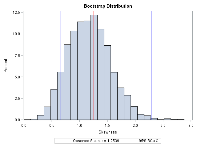
The bootstrap distribution tells you how the statistic (in this case, the skewness) might vary due to random sampling variation. You can use a histogram to visualize the bootstrap distribution of the skewness statistic:
title "Bootstrap Distribution"; %let Est = 0.366; proc sgplot data=OutStats; label Skewness= ; histogram Skewness; /* Optional: draw reference line at observed value and draw 95% CI */ refline &Est / axis=x lineattrs=(color=red) name="Est" legendlabel="Observed Statistic = &Est"; refline -0.44737 0.96934 / axis=x lineattrs=(color=blue) name="CI" legendlabel="95% CI"; keylegend "Est" "CI"; run; |
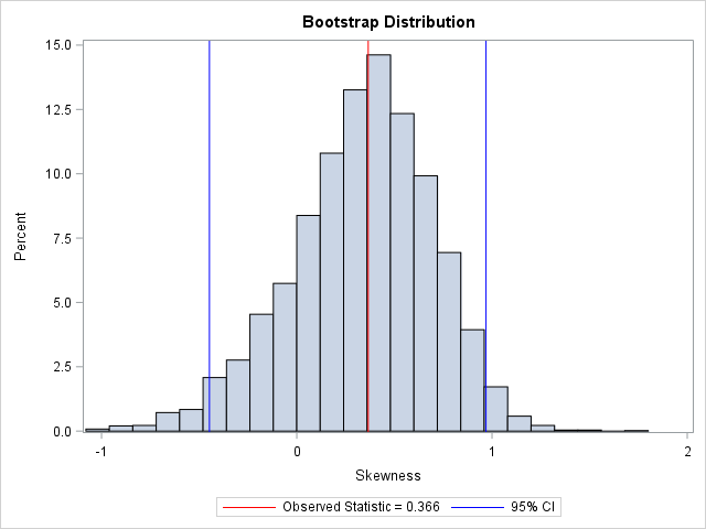
In this graph, the REFLINE statement is used to display (in red) the observed value of the statistic for the original data. A second REFLINE statement plots (in blue) an approximate 95% confidence interval for the skewness parameter, which is computed in the next section. The bootstrap confidence interval contains 0, thus you cannot conclude that the skewness parameter is significantly different from 0.
Compute a bootstrap confidence interval in SAS
The standard deviation of the bootstrap distribution is an estimate for the standard error of the statistic. If the sampling distribution is approximately normal, you can use this fact to construct the usual Wald confidence interval about the observed value of the statistic. That is, if T is the observed statistic, then
the endpoints of the 95% two-sided confidence interval are T ± 1.96 SE. (Or use the so-called bootstrap t interval by replacing 1.96 with tα/2, n-1.) The following call to PROC MEANS produces the standard error (not shown):
proc means data=OutStats nolabels N StdDev; var Skewness; run; |
However, since the bootstrap distribution is an approximate sampling distribution, you don’t need to rely on a normality assumption. Instead, you can use percentiles of the bootstrap distribution to estimate a confidence interval. For example, the following call to PROC UNIVARIATE computes a two-side 95% confidence interval by using the lower 2.5th percentile and the upper 97.5th percentile of the bootstrap distribution:
/* 4. Use approx sampling distribution to make statistical inferences */ proc univariate data=OutStats noprint; var Skewness; output out=Pctl pctlpre =CI95_ pctlpts =2.5 97.5 /* compute 95% bootstrap confidence interval */ pctlname=Lower Upper; run; proc print data=Pctl noobs; run; |
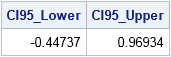
As mentioned previously, the 95% bootstrap confidence interval contains 0. Although the observed skewness value (0.366) might not seem very close to 0, the bootstrap distribution shows that there is substantial variation in the skewness statistic in small samples.
The bootstrap percentile method is a simple way to obtain a confidence interval for many statistics. There are several more sophisticated methods for computing a bootstrap confidence interval, but this simple method provides an easy way to use the bootstrap to assess the accuracy of a point estimate. For an overivew of bootstrap methods, see Davison and Hinkley (1997) Bootstrap Methods and their Application.
tags: Bootstrap and Resampling
The post Compute a bootstrap confidence interval in SAS appeared first on The DO Loop.
| This post was kindly contributed by The DO Loop - go there to comment and to read the full post. |
↧
The smooth bootstrap method in SAS
| This post was kindly contributed by The DO Loop - go there to comment and to read the full post. |
Last week I showed how to use the simple bootstrap to randomly resample from the data to create B bootstrap samples, each containing N observations.
The simple bootstrap is equivalent to sampling from the empirical cumulative distribution function (ECDF) of the data. An alternative bootstrap technique is called the smooth bootstrap. In the smooth bootstrap you add a small amount of random noise to each observation that
is selected during the resampling process. This is equivalent to sampling from a kernel density
estimate, rather than from the empirical density.
The example in this article is adapted from Chapter 15 of Wicklin (2013), Simulating Data with SAS.
The bootstrap method in SAS/IML
My previous article used the bootstrap method to investigate the sampling distribution of the skewness statistic for the SepalWidth variable in the Sashelp.Iris data. I used PROC SURVEYSELECT to resample the data and used PROC MEANS to analyze properties of the bootstrap distribution. You can also use SAS/IML to implement the bootstrap method.
The following SAS/IML statements creates 5000 bootstrap samples of the SepalWidth data. However, instead of computing a bootstrap distribution for the skewness statistic, this program computes a bootstrap distribution for the median statistic. The SAMPLE function enables you to resample from the data.
data sample(keep=x);
set Sashelp.Iris(where=(Species="Virginica") rename=(SepalWidth=x));
run;
/* Basic bootstrap confidence interval for median */
%let NumSamples = 5000; /* number of bootstrap resamples */
proc iml;
use Sample; read all var {x}; close Sample; /* read data */
call randseed(12345); /* set random number seed */
obsStat = median(x); /* compute statistic on original data */
s = sample(x, &NumSamples // nrow(x)); /* bootstrap samples: 50 x NumSamples */
D = T( median(s) ); /* bootstrap distribution for statistic */
call qntl(q, D, {0.025 0.975}); /* basic 95% bootstrap CI */
results = obsStat || q`;
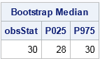
print results[L="Bootstrap Median" c={"obsStat" "P025" "P975"}];
|
The SAS/IML program is very compact. The MEDIAN function computes the median for the original data. The SAMPLE function generates 5000 resamples; each bootstrap sample is a column of the s matrix.
The MEDIAN function then computes the median of each column. The QNTL subroutine computes a 95% confidence interval for the median as [28, 30]. (Incidentally, you can use PROC UNIVARIATE to compute distribution-free confidence intervals for standard percentiles such as the median.)
The bootstrap distribution of the median
The following statement create a histogram of the bootstrap distribution of the median:
title "Bootstrap Distribution for Median"; call histogram(D) label="Median"; /* create histogram in SAS/IML */ |
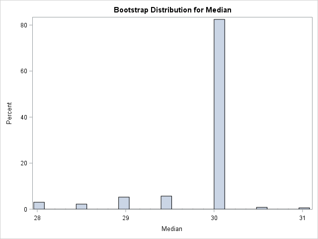
I was surprised when I first saw a bootstrap distribution like this. The distribution contains discrete values. More than 80% of the bootstrap samples have a median value of 30. The remaining samples have values that are integers or half-integers.
This distribution is typical of the bootstrap distribution for a percentile. Three factors contribute to the shape:
- The measurements are rounded to the nearest millimeter. Thus the data are discrete integers.
- The sample median is always a data value or (for N even) the midpoint between two data values. In fact, this statement is true for all percentiles.
- In the Sample data, the value 30 is not only the median, but is the mode. Consequently, many bootstrap samples will have 30 as the median value.
The smooth bootstrap can analyze percentiles of rounded data #StatWisdom #SASTip
Click To Tweet
Smooth bootstrap
Although the bootstrap distribution for the median is correct, it is somewhat unsatisfying.
Widths and lengths represent continuous quantities. Consequently, the true sampling distribution of the median statistic is continuous.
The bootstrap distribution would look more continuous if the data had been measured with more precision. Although you cannot change the data, you can change the way that you create bootstrap samples. Instead of drawing resamples from the (discrete) ECDF, you can randomly draw samples from a kernel density estimate (KDE) of the data. The resulting samples will not contain data values. Instead, they will contains values that are randomly drawn from a continuous KDE.
You have to make two choices for the KDE: the shape of the kernel and the bandwidth. This article explores two possible choices:
- Uniform kernel: A recorded measurement of 30 mm means that the true value of the sepal was in the interval [29.5, 30.5). In general, a recorded value of x means that the true value is in [x-0.5, x+0.5). Assuming that any point in that interval is equally likely leads to a uniform kernel with bandwidth 0.5.
- Normal kernel: You can assume that the true measurement is normally distributed, centered on the measured value, and is very likely to be within [x-0.5, x+0.5). For a normal distribution, 95% of the probability is contained in ±2σ of the mean, so you could choose σ=0.25 and assume that the true value for the measurement x is in the distribution N(x, 0.25).
For more about the smooth bootstrap, see Davison and Hinkley (1997) Bootstrap Methods and their Application.
Smooth bootstrap in SAS/IML
For the iris data, the uniform kernel seems intuitively appealing. The following SAS/IML program defines a function named SmoothUniform that randomly chooses B samples and adds a random U(-h, h) variate to each data point. The medians of the columns form the bootstrap distribution.
/* randomly draw a point from x. Add noise from U(-h, h) */
start SmoothUniform(x, B, h);
   N = nrow(x) * ncol(x);
   s = Sample(x, N // B);               /* B x N matrix */
   eps = j(B, N);                       /* allocate vector */
   call randgen(eps, "Uniform", -h, h); /* fill vector */
   return( s + eps );                   /* add random uniform noise */
finish;

s = SmoothUniform(x, &NumSamples, 0.5); /* columns are bootstrap samples from KDE */
D = T( median(s) );                     /* median of each col is bootstrap distrib */
BSEst = mean(D);                        /* bootstrap estimate of median */
call qntl(q, D, {0.025 0.975});         /* basic 95% bootstrap CI */
results = BSEst || q`;
print results[L="Smooth Bootstrap (Uniform Kernel)" c={"Est" "P025" "P975"}];
|
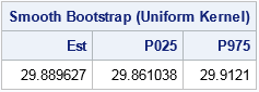
The smooth bootstrap distribution (not shown) is continuous.
The mean of the distribution is the bootstrap estimate for the median. The estimate for this run is 29.8. The central 95% of the smooth bootstrap distribution is [29.77, 29.87]. The bootstrap estimate is close to the observed median, but the CI is much smaller than the earlier simple CI. Notice that the observed median (which is computed on the rounded data) is not in the 95% CI from the smooth bootstrap distribution.
Many researchers in density estimation state that the shape of the kernel function does not have a strong impact on the density estimate (Scott (1992), Multivariate Density Estimation, p. 141). Nevertheless, the following SAS/IML statements define a function called SmoothNormal that implements a smoothed bootstrap with a normal kernel:
/* Smooth bootstrap with normal kernel and sigma = h */ start SmoothNormal(x, B, h); N = nrow(x) * ncol(x); s = Sample(x, N // B); /* B x N matrix */ eps = j(B, N); /* allocate vector */ call randgen(eps, "Normal", 0, h); /* fill vector */ return( s + eps ); /* add random normal variate */ finish; s = SmoothNormal(x, &NumSamples, 0.25); /* bootstrap samples from KDE */ |
The mean of this smooth bootstrap distribution is
29.89. The central 95% interval is [29.86, 29.91]. As expected, these values are similar to the values obtained by using the uniform kernel.
Summary of the smooth bootstrap
In summary, the SAS/IML language provides a compact and efficient way to implement the bootstrap method for a univariate statistic such as the skewness or median. A visualization of the bootstrap distribution of the median reveals that the distribution is discrete due to the rounded data values and the statistical properties of percentiles. If you choose, you can “undo” the rounding by implementing the smooth bootstrap method. The smooth bootstrap is equivalent to drawing bootstrap samples from a kernel density estimate of the data. The resulting bootstrap distribution is continuous and gives a smaller confidence interval for the median of the population.
tags: Bootstrap and Resampling
The post The smooth bootstrap method in SAS appeared first on The DO Loop.
| This post was kindly contributed by The DO Loop - go there to comment and to read the full post. |
↧
↧
The jackknife method to estimate standard errors in SAS
| This post was kindly contributed by The DO Loop - go there to comment and to read the full post. |
One way to assess the precision of a statistic (a point estimate) is to compute the standard error, which is the standard deviation of the statistic’s sampling distribution. A relatively large standard error indicates that the point estimate should be viewed with skepticism, either because the sample size is small or because the data themselves have a large variance.
The jackknife method is one way to estimate the standard error of a statistic.
Some simple statistics have explicit formulas for the standard error, but the formulas often assume normality of the data or a very large sample size. When your data do not satisfy the assumptions or when no formula exists, you can use resampling techniques to estimate the standard error. Bootstrap resampling is one choice, and the jackknife method is another. Unlike the bootstrap, which uses random samples, the jackknife is a deterministic method.
This article explains the jackknife method and describes how to compute jackknife estimates in SAS/IML software.
This is best when the statistic that you need is also implemented in SAS/IML. If the statistic is computed by a SAS procedure, you might prefer to download and use the %JACK macro, which does not require SAS/IML.
The jackknife method: Leave one out!
The jackknife method estimates the standard error (and bias) of statistics without making any parametric assumptions about the population that generated the data. It uses only the sample data.
The jackknife method manufactures jackknife samples from the data.
A jackknife sample is a “leave-one-out” resample of the data. If there are n observations, then there are n jackknife samples, each of size n-1. If the original data are
{x1, x2,…, xn},
then the i_th jackknife sample is
{x1,…, xi-1,xi+1,…, xn}
You then compute n jackknife replicates. A jackknife replicate is the statistic of interest computed on a jackknife sample. You can obtain an estimate of the standard error from the variance of the jackknife replicates. The jackknife method is summarized by the following:
- Compute a statistic, T, on the original sample of size n.
- For i = 1 to n, repeat the following:
- Leave out the i_th observation to form the i_th jackknife sample.
- Compute the i_th jackknife replicate statistic, Ti, by computing the statistic on the i_th jacknife sample.
Tavg)**2 )
Data for a jackknife example
Resampling methods are not hard, but the notation in some books can be confusing. To clarify the method, let’s choose a particular statistic and look at example data. The following example is from Martinez and Martinez (2001, 1st Ed, p. 241), which is also the source for this article. The data are the LSAT scores and grade-point averages (GPAs) for 15 randomly chosen students who applied to law school.
data law; input lsat gpa @@; datalines; 653 3.12 576 3.39 635 3.30 661 3.43 605 3.13 578 3.03 572 2.88 545 2.76 651 3.36 555 3.00 580 3.07 594 2.96 666 3.44 558 2.81 575 2.74 ; |
The statistic of interest (T) will be the correlation coefficient between the LSAT and the GPA variables for the n=15 observations. The observed correlation is TData = 0.776. The standard error of T helps us understand how much T would change if we took a different random sample of 15 students.
The next sections show how to implement the jackknife analysis in the SAS/IML language.
Construct a jackknife sample in SAS
The SAS/IML matrix language is the simplest way to perform a general jackknife estimates. If X is an n x p data matrix, you can obtain the i_th jackknife sample by excluding the i_th row of X. The following two helper functions encapsulate some of the computations. The SeqExclude function returns the index vector {1, 2, …, i-1, i+1, …, n}. The JackSample function returns the data matrix without the i_th row:
proc iml; /* return the vector {1,2,...,i-1, i+1,...,n}, which excludes the scalar value i */ start SeqExclude(n,i); if i=1 then return 2:n; if i=n then return 1:n-1; return (1:i-1) || (i+1:n); finish; /* return the i_th jackknife sample for (n x p) matrix X */ start JackSamp(X,i); n = nrow(X); return X[ SeqExclude(n, i), ]; /* return data without i_th row */ finish; |
The jackknife method for multivariate data in SAS
By using the helper functions, you can carry out each step of the jackknife method. To make the method easy to modify for other statistics, I’ve written a function called EvalStat which computes the correlation coefficient. This function is called on the original data and on each jackknife sample.
/* compute the statistic in this function */ start EvalStat(X); return corr(X)[2,1]; /* <== Example: return correlation between two variables */ finish; /* read the data into a (n x 2) data matrix */ use law; read all var {"gpa" "lsat"} into X; close; /* 1. compute statistic on observed data */ T = EvalStat(X); /* 2. compute same statistic on each jackknife sample */ n = nrow(X); T_LOO = j(n,1,.); /* LOO = "Leave One Out" */ do i = 1 to n; Y = JackSamp(X,i); T_LOO[i] = EvalStat(Y); end; /* 3. compute mean of the LOO statistics */ T_Avg = mean( T_LOO ); /* 4 & 5. compute jackknife estimates of bias and standard error */ biasJack = (n-1)*(T_Avg - T); stdErrJack = sqrt( (n-1)/n * ssq(T_LOO - T_Avg) ); result = T || T_Avg || biasJack || stdErrJack; print result[c={"Estimate" "Mean Jackknife Estimate" "Bias" "Std Error"}]; |

The output shows that the estimate of bias for the correlation coefficient is very small. The standard error of the correlation coefficient is estimated as 0.14, which is about 18% of the estimate.
To use this code yourself, simply modify the EvalStat function. The remainder of the program does not need to change.
The jackknife method in SAS/IML: Univariate data
When the data are univariate, you can sometimes eliminate the loop that computes jackknife samples and evaluates the jackknife replicates.
If X is column vector, you can computing the (n-1) x n matrix whose i_th column represents the i_th jackknife sample. (To prevent huge matrices, this method is best for n < 20000.)
Because many statistical functions in SAS/IML operate on the columns of a matrix, you can often compute the jackknife replicates in a vectorized manner.
In the following program, the JackSampMat function returns the matrix of jackknife samples for univariate data. The function calls the REMOVE function in SAS/IML, which deletes specified elements of a matrix and returns the results in a row vector. The EvalStatMat function takes the matrix of jackknife samples and returns a row vector of statistics, one for each column. In this example, the function returns the sample standard deviation.
/* If x is univariate, you can construct a matrix where each column contains a jackknife sample. Use for univariate column vector x when n < 20000 */ start JackSampMat(x); n = nrow(x); B = j(n-1, n,0); do i = 1 to n; B[,i] = remove(x, i)`; /* transpose to column vevtor */ end; return B; finish; /* Input: matrix where each column of X is a bootstrap sample. Return a row vector of statistics, one for each column. */ start EvalStatMat(x); return std(x); /* <== Example: return std dev of each sample */ finish; |
Let’s use these functions to get a jackknife estimate of the standard error for the statistic (the standard deviation). The data (from Martinez and Martinez, p. 246) have been studied by many researchers and represent the weight gain in grams for 10 rats who were fed a low-protein diet of cereal:
x = {58,67,74,74,80,89,95,97,98,107}; /* Weight gain (g) for 10 rats */ /* optional: visualize the matrix of jackknife samples */ *M = JackSampMat(x); *print M[c=("S1":"S10") r=("1":"9")]; /* Jackknife method for univariate data */ /* 1. compute observed statistic */ T = EvalStatMat(x); /* 2. compute same statistic on each jackknife sample */ T_LOO = EvalStatMat( JackSampMat(x) ); /* LOO = "Leave One Out" */ /* 3. compute mean of the LOO statistics */ T_Avg = mean( T_LOO` ); /* transpose T_LOO */ /* 4 & 5. compute jackknife estimates of bias and standard error */ biasJack = (n-1)*(T_Avg - T); stdErrJack = sqrt( (n-1)/n * ssq(T_LOO - T_Avg) ); result = T || T_Avg || biasJack || stdErrJack; print result[c={"Estimate" "Mean Jackknife Estimate" "Bias" "Std Error"}]; |

The output shows that the standard deviation of these data is about 15.7 grams. The jackknife method computes that the standard error for this statistic about 2.9 grams, which is about 18% of the estimate.
In summary, jackknife estimates are straightforward to implement in SAS/IML. This article shows a general implementation that works for all data and a specialized implementation that works for univariate data. In both cases, you can adapt the code for your use by modifying the function that computes the statistic on a data set. This approach is useful and efficient when the statistic is implemented in SAS/IML.
The post The jackknife method to estimate standard errors in SAS appeared first on The DO Loop.
| This post was kindly contributed by The DO Loop - go there to comment and to read the full post. |
↧
Bootstrap estimates in SAS/IML
| This post was kindly contributed by The DO Loop - go there to comment and to read the full post. |
I previously wrote about how to compute a bootstrap confidence interval in Base SAS. As a reminder, the bootstrap method consists of the following steps:
- Compute the statistic of interest for the original data
- Resample B times from the data to form B bootstrap samples. B is usually a large number, such as B = 5000.
- Compute the statistic on each bootstrap sample. This creates the bootstrap distribution, which approximates the sampling distribution of the statistic.
- Use the bootstrap distribution to obtain bootstrap estimates such as standard errors and confidence intervals.
In my book Simulating Data with SAS, I describe efficient ways to bootstrap in the SAS/IML matrix language. Whereas the Base SAS implementation of the bootstrap requires calls to four or five procedure, the SAS/IML implementation requires only a few function calls. This article shows how to compute a bootstrap confidence interval from percentiles of the bootstrap distribution for univariate data. How to bootstrap multivariate data is discussed on p. 189 of Simulating Data with SAS.
Skewness of univariate data
Let’s use the bootstrap to find a 95% confidence interval for the skewness statistic. The data are the petal widths of a sample of 50 randomly selected flowers of the species Iris setosa. The measurements (in mm) are contained in the data set Sashelp.Iris.
So that you can easily generalize the code to other data, the following statements create a data set called SAMPLE and the rename the variable to analyze to ‘X’. If you do the same with your data, you should be able to reuse the program by modifying only a few statements.
The following DATA step renames the data set and the analysis variable. A call to PROC UNIVARIATE graphs the data and provides a point estimate of the skewness:
data sample; set sashelp.Iris; /* <== load your data here */ where species = "Setosa"; rename PetalWidth=x; /* <== rename the analyzes variable to 'x' */ run; proc univariate data=sample; var x; histogram x; inset N Skewness (6.3) / position=NE; run; |
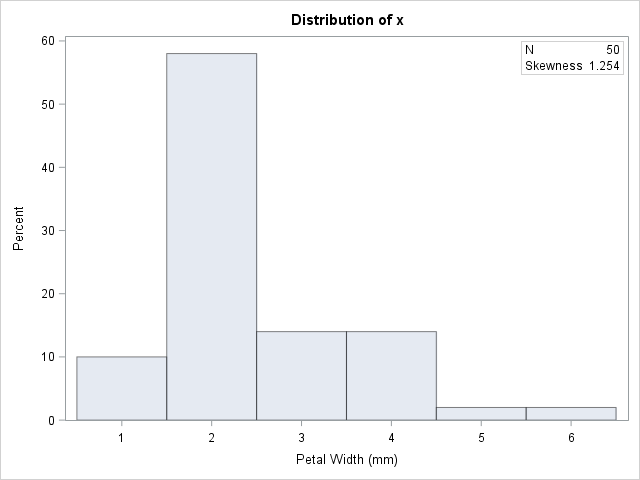
The petal widths have a highly skewed distribution, with a skewness estimate of 1.25.
A bootstrap analysis in SAS/IML
Running a bootstrap analysis in SAS/IML requires only a few lines to compute the confidence interval, but to help you generalize the problem to statistics other than the skewness, I wrote a function called EvalStat. The input argument is a matrix where each column is a bootstrap sample. The function returns a row vector of statistics, one for each column. (For the skewness statistic, the EvalStat function is a one-liner.) The EvalStat function is called twice: once on the original column vector of data and again on a matrix that contains bootstrap samples in each column. You can create the matrix by calling the SAMPLE function in SAS/IML, as follows:
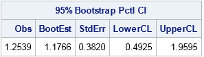
/* Basic bootstrap percentile CI. The following program is based on Chapter 15 of Wicklin (2013) Simulating Data with SAS, pp 288-289. */ proc iml; /* Function to evaluate a statistic for each column of a matrix. Return a row vector of statistics, one for each column. */ start EvalStat(M); return skewness(M); /* <== put your computation here */ finish; alpha = 0.05; B = 5000; /* B = number of bootstrap samples */ use sample; read all var "x"; close; /* read univariate data into x */ call randseed(1234567); Est = EvalStat(x); /* 1. compute observed statistic */ s = sample(x, B // nrow(x)); /* 2. generate many bootstrap samples (N x B matrix) */ bStat = T( EvalStat(s) ); /* 3. compute the statistic for each bootstrap sample */ bootEst = mean(bStat); /* 4. summarize bootstrap distrib such as mean, */ SE = std(bStat); /* standard deviation, */ call qntl(CI, bStat, alpha/2 || 1-alpha/2); /* and 95% bootstrap percentile CI */ R = Est || BootEst || SE || CI`; /* combine results for printing */ print R[format=8.4 L="95% Bootstrap Pctl CI" c={"Obs" "BootEst" "StdErr" "LowerCL" "UpperCL"}]; |
The SAS/IML program for the bootstrap is very compact. It is important to keep track of the dimensions of each variable. The EST, BOOTEST, and SE variables are scalars. The S variable is a B x N matrix, where N is the sample size. The BSTAT variable is a column vector with N elements. The CI variable is a two-element column vector.
The output summarizes the bootstrap analysis. The estimate for the skewness of the observed data is 1.25. The bootstrap distribution (the skewness of the bootstrap samples) enables you to estimate three common quantities:
- The bootstrap estimate of the skewness is 1.18. This value is computed as the mean of the bootstrap distribution.
- The bootstrap estimate of the standard error of the skewness is 0.38. This value is computed as the standard deviation of the bootstrap distribution.
- The bootstrap percentile 95% confidence interval is computed as the central 95% of the bootstrap estimates, which is the interval
[0.49, 1.96].
It is important to realize that these estimate will vary slightly if you use different random-number seeds or a different number of bootstrap iterations (B).
You can visualize the bootstrap distribution by drawing a histogram of the bootstrap estimates. You can overlay the original estimate (or the bootstrap estimate) and the endpoints of the confidence interval, as shown below.

In summary, you can implement the bootstrap method in the SAS/IML language very compactly.
You can use the bootstrap distribution to estimate the
parameter and standard error.
The bootstrap percentile method, which is based on quantiles of the bootstrap distribution, is a simple way to obtain a confidence interval for a parameter.
You can download the full SAS program that implements this analysis.
The post Bootstrap estimates in SAS/IML appeared first on The DO Loop.
| This post was kindly contributed by The DO Loop - go there to comment and to read the full post. |
↧
The bias-corrected and accelerated (BCa) bootstrap interval
| This post was kindly contributed by The DO Loop - go there to comment and to read the full post. |
I recently showed how to compute a bootstrap percentile confidence interval in SAS.
The percentile interval is a simple “first-order” interval that is formed from quantiles of the bootstrap distribution. However, it has two limitations. First, it does not use the estimate for the original data; it is based only on bootstrap resamples. Second, it does not adjust for skewness in the bootstrap distribution. The so-called bias-corrected and accelerated bootstrap interval (the BCa interval) is a second-order accurate interval that addresses these issues. This article shows how to compute the BCa bootstrap interval in SAS. You can
download the complete SAS program that implements the BCa computation.
As in the previous article, let’s bootstrap the skewness statistic for the petal widths of 50 randomly selected flowers of the species Iris setosa. The following statements create a data set called SAMPLE and the rename the variable to analyze to ‘X’, which is analyzed by the rest of the program:
data sample; set sashelp.Iris; /* <== load your data here */ where species = "Setosa"; rename PetalWidth=x; /* <== rename the analyzes variable to 'x' */ run; |
BCa interval: The main ideas
The main advantage to the BCa interval is that it corrects for bias and skewness in the distribution of bootstrap estimates.
The BCa interval requires that you estimate two parameters. The bias-correction parameter, z0, is related to the proportion of bootstrap estimates that are less than the observed statistic. The acceleration parameter, a, is proportional to the skewness of the bootstrap distribution. You can use the jackknife method to estimate the acceleration parameter.
Assume that the data are independent and identically distributed.
Suppose that you have already computed the original statistic and a large number of bootstrap estimates, as shown in the previous article. To compute a BCa confidence interval, you estimate z0 and a and use them to adjust the endpoints of the percentile confidence interval (CI). If the bootstrap distribution is positively skewed, the CI is adjusted to the right. If the bootstrap distribution is negatively skewed, the CI is adjusted to the left.
Estimate the bias correction and acceleration
The mathematical details of the BCa adjustment are provided in Chernick and LaBudde (2011)
and Davison and Hinkley (1997). My computations were inspired by Appendix D of Martinez and Martinez (2001). To make the presentation simpler, the program analyzes only univariate data.
The bias correction factor is related to the proportion of bootstrap estimates that are less than the observed statistic. The acceleration parameter is proportional to the skewness of the bootstrap distribution. You can use the jackknife method to estimate the acceleration parameter. The following SAS/IML modules encapsulate the necessary computations. As described in the jackknife article, the function ‘JackSampMat’ returns a matrix whose columns contain the jackknife samples and the function ‘EvalStat’ evaluates the statistic on each column of a matrix.
proc iml; load module=(JackSampMat); /* load helper function */ /* compute bias-correction factor from the proportion of bootstrap estimates that are less than the observed estimate */ start bootBC(bootEst, Est); B = ncol(bootEst)*nrow(bootEst); /* number of bootstrap samples */ propLess = sum(bootEst < Est)/B; /* proportion of replicates less than observed stat */ z0 = quantile("normal", propLess); /* bias correction */ return z0; finish; /* compute acceleration factor, which is related to the skewness of bootstrap estimates. Use jackknife replicates to estimate. */ start bootAccel(x); M = JackSampMat(x); /* each column is jackknife sample */ jStat = EvalStat(M); /* row vector of jackknife replicates */ jackEst = mean(jStat`); /* jackknife estimate */ num = sum( (jackEst-jStat)##3 ); den = sum( (jackEst-jStat)##2 ); ahat = num / (6*den##(3/2)); /* ahat based on jackknife ==> not random */ return ahat; finish; |
Compute the BCa confidence interval
With those helper functions defined, you can compute the BCa confidence interval. The following SAS/IML statements read the data, generate the bootstrap samples, compute the bootstrap distribution of estimates, and compute the 95% BCa confidence interval:
/* Input: matrix where each column of X is a bootstrap sample. Return a row vector of statistics, one for each column. */ start EvalStat(M); return skewness(M); /* <== put your computation here */ finish; alpha = 0.05; B = 5000; /* B = number of bootstrap samples */ use sample; read all var "x"; close; /* read univariate data into x */ call randseed(1234567); Est = EvalStat(x); /* 1. compute observed statistic */ s = sample(x, B // nrow(x)); /* 2. generate many bootstrap samples (N x B matrix) */ bStat = T( EvalStat(s) ); /* 3. compute the statistic for each bootstrap sample */ bootEst = mean(bStat); /* 4. summarize bootstrap distrib, such as mean */ z0 = bootBC(bStat, Est); /* 5. bias-correction factor */ ahat = bootAccel(x); /* 6. ahat = acceleration of std error */ print z0 ahat; /* 7. adjust quantiles for 100*(1-alpha)% bootstrap BCa interval */ zL = z0 + quantile("normal", alpha/2); alpha1 = cdf("normal", z0 + zL / (1-ahat*zL)); zU = z0 + quantile("normal", 1-alpha/2); alpha2 = cdf("normal", z0 + zU / (1-ahat*zU)); call qntl(CI, bStat, alpha1//alpha2); /* BCa interval */ R = Est || BootEst || CI`; /* combine results for printing */ print R[c={"Obs" "BootEst" "LowerCL" "UpperCL"} format=8.4 L="95% Bootstrap Bias-Corrected CI (BCa)"]; |
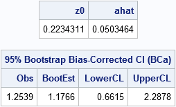
The BCa interval is [0.66, 2.29].
For comparison, the bootstrap percentile CI for the bootstrap distribution, which was computed in the previous bootstrap article, is [0.49, 1.96].
Notice that by using the bootBC and bootAccel helper functions, the program is compact and easy to read. One of the advantages of the SAS/IML language is the ease with which you can define user-defined functions that encapsulate sub-computations.
You can visualize the analysis by plotting the bootstrap distribution overlaid with the observed statistic and the 95% BCa confidence interval. Notice that the BCa interval is not symmetric about the bootstrap estimate. Compared to the bootstrap percentile interval (see the previous article), the BCa interval is shifted to the right.
There is another second-order method that is related to the BCa interval. It is called the ABC method and it uses an analytical expression to approximate the endpoints of the BCa interval. See p. 214 of Davison and
Hinkley (1997).
In summary, bootstrap computations in the SAS/IML language can be very compact. By writing and re-using helper functions, you can encapsulate some of the tedious calculations into a high-level function, which makes the resulting program easier to read. For univariate data, you can often implement bootstrap computations without writing any loops by using the matrix-vector nature of the SAS/IML language.
If you do not have access to SAS/IML software or if the statistic that you want to bootstrap is produced by a SAS procedure, you can use SAS-supplied macros (%BOOT, %JACK,…) for bootstrapping. The macros include the %BOOTCI macro, which supports the percentile interval, the BCa interval, and others. For further reading, the web page for the macros includes a comparison of the CI methods.
The post The bias-corrected and accelerated (BCa) bootstrap interval appeared first on The DO Loop.
| This post was kindly contributed by The DO Loop - go there to comment and to read the full post. |
↧
The top 10 posts from The DO Loop in 2017
| This post was kindly contributed by The DO Loop - go there to comment and to read the full post. |
I wrote more than 100 posts for The DO Loop blog in 2017.
The most popular articles were about SAS programming tips, statistical data analysis, and simulation and bootstrap methods.
Here are the most popular articles from 2017 in each category.
General SAS programming techniques
-
INTCK and INTNX:
Do you use dates in SAS? Then you’ve probably needed to compute the number of time intervals (days, weeks, years) between two dates or the date that is a specified number of time intervals before or after a given date.
The INTCK and INTNX functions in SAS make these date-related tasks easy. -
PUT and %PUT:
The PUT and %PUT statements are two of the simplest statements in SAS. They write information to the SAS log. This post shows how to get the PUT and %PUT statements to display arrays, name-value pairs, and more. -
LEAVE and CONTINUE:
An iterative loop is one of the simplest programming constructs. Did you know that you can use the LEAVE and CONTINUE statements in SAS to exit a DO loop or go immediately to the next iteration when some condition is satisfied? -
ODS OUTPUT:
The ODS OUTPUT statement enables you to store any value that is produced by any SAS procedure. You can then read that value by using a SAS program. This is a highly useful tool for statistical programmers.
Statistics and Data Analysis

-
M&M Colors:
It’s no surprise that a statistical analysis of the color distribution of M&M candies was one of the most popular articles. Some people are content to know that the candies are delicious, but thousands wanted to read about whether blue and orange candies occur more often than brown. -
Interpretation of Correlation:
Correlation is one of the simplest multivariate statistics, but it can be interpreted in many ways: algebraic, geometric, in terms of regression, and more.
This article describes seven ways to view correlation? -
Winsorize Data:
Before you ask “how can I Winsorize data” to eliminate outliers, you should ask “what is Winsorization” and “what are the pitfalls?” This article presents the advantages and disadvantages of Winsorizing data.
Simulation and Bootstrapping
-
Choose a random number seed:
How should you choose a seed value to initialize a random-number generator? Are some seeds “more random than others”? Should you use your birthday or phone number? This article discusses how to choose a seed for generating random numbers. -
Run 1000 Regression Models:
In data analysis, you might need to run many one-variable regression models. This situation also arises in simulation studies. Regardless of the source of the data, this article shows how to run thousands of regression models without using a macro loop. -
Construct a BCa Interval:
Sometimes I can predict that an article will be popular. Other times I am surprised. I did not anticipate that thousands of people would want to read about how to construct a bias-corrected and accelerated (BCa) bootstrap interval in SAS.
Was your New Year’s resolution to learn more about SAS?
Did you miss any of these popular posts? Take a moment to read (or re-read!) one of these top 10 posts from the past year.
The post The top 10 posts from <em>The DO Loop</em> in 2017 appeared first on The DO Loop.
| This post was kindly contributed by The DO Loop - go there to comment and to read the full post. |
↧
↧
Sample and obtain the results in random order
| This post was kindly contributed by The DO Loop - go there to comment and to read the full post. |
The SURVEYSELECT procedure in SAS 9.4M5 supports the OUTRANDOM option, which causes the selected items in a simple random sample to be randomly permuted after they are selected.
This article describes several statistical tasks that benefit from this option, including simulating card games, randomly permuting observations in a DATA step, assigning a random ID to patients in a clinical study, and generating bootstrap samples.
In each case, the new OUTRANDOM option reduces the number of statements that you need to write. The OUTRANDOM option can also be specified by using
OUTORDER=RANDOM.
Sample data with PROC SURVEYSELECT
Often when you draw a random sample (with or without replacement) from a population, the order in which the items were selected is not important. For example, if you have 10 patients in a clinical trial and want to randomly assign five patients to the control group, the control group does not depend on the order in which the patients were selected. Similarly, in simulation studies, many statistics (means, proportions, standard deviations,…) depend only on the sample, not on the order in which the sample was generated.
For these reasons, and for efficiency, the SURVEYSELECT procedure in SAS uses a “one-pass” algorithm to select observations in the same order that they appear in the “population” data set.
However, sometimes you might require the output data set from PROC SURVEYSELECT to be in a random order. For example, in a poker simulation, you might want the output of PROC SURVEYSELECT to represent a random shuffling of the 52 cards in a deck.
To be specific, the following DATA step generates a deck of 52 cards in order: Aces first, then 2s, and so on up to jacks, queens, and kings. If you use PROC SURVEYSELECT and METHOD=SRS to select 10 cards at random (without replacement), you obtain the following subset:
data CardDeck; length Face $2 Suit $8; do Face = 'A','2','3','4','5','6','7','8','9','10','J','Q','K'; do Suit = 'Clubs', 'Diamonds', 'Hearts', 'Spades'; CardNumber + 1; output; end; end; run; /* Deal 10 cards. Order is determined by input data */ proc surveyselect data=CardDeck out=Deal noprint seed=1234 method=SRS /* sample w/o replacement */ sampsize=10; /* number of observations in sample */ run; proc print data=Deal; run; |

Notice that the call to PROC SURVEYSELECT did not use the OUTRANDOM option. Consequently, the cards are in the same order as they appear in the input data set.
This sample is adequate if you want to simulate dealing hands and estimate probabilities of pairs, straights, flushes, and so on. However, if your simulation requires the cards to be in a random order (for example, you want the first five observations to represent the first player’s cards), then clearly this sample is inadequate and needs an additional random permutation of the observations.
That is exactly what the OUTRANDOM option provides, as shown by the following call to PROC SURVEYSELECT:
/* Deal 10 cards in random order */ proc surveyselect data=CardDeck out=Deal2 noprint seed=1234 method=SRS /* sample w/o replacement */ sampsize=10 /* number of observations in sample */ OUTRANDOM; /* SAS/STAT 14.3: permute order */ run; proc print data=Deal2; run; |

You can use this sample when the output needs to be in a random order. For example, in a poker simulation, you can now assign the first five cards to the first player and the second five cards to a second player.
Permute the observations in a data set
A second application of the OUTRANDOM option is to permute the rows of a SAS data set. If you sample without replacement and request all observations (SAMPRATE=1), you obtain a copy of the original data in random order. For example, the students in the Sashelp.Class data set are listed in alphabetical order by their name. The following statements use the OUTRANDOM option to rearrange the students in a random order:
/* randomly permute order of observations */ proc surveyselect data=Sashelp.Class out=RandOrder noprint seed=123 method=SRS /* sample w/o replacement */ samprate=1 /* proportion of observations in sample */ OUTRANDOM; /* SAS/STAT 14.3: permute order */ run; proc print data=RandOrder; run; |

There are many other ways to permute the rows of a data set, such as adding a uniform random variable to the data and then sorting. The two methods are equivalent, but the code for the SURVEYSELECT procedure is shorter to write.
Assign unique random IDs to patients in a clinical trial
Another application of the OUTRANDOM option is to assign a unique random ID to participants in an experimental trial. For example, suppose that four-digit integers are used for an ID variable. Some clinical trials assign an ID number sequentially to each patient in the study, but I recently learned from a SAS discussion forum that some companies assign random ID values to subjects. One way to assign random IDs is to sample randomly without replacement from the set of all ID values. The following DATA step generates all four-digit IDs, selects 19 of them in random order, and then merges those IDs with the participants in the study:
data AllIDs; do ID = 1000 to 9999; /* create set of four-digit ID values */ output; end; run; /* randomly select 19 unique IDs */ proc surveyselect data=AllIDs out=ClassIDs noprint seed=12345 method=SRS /* sample w/o replacement */ sampsize=19 /* number of observations in sample */ OUTRANDOM; /* SAS/STAT 14.3: permute order */ run; data Class; merge ClassIDs Sashelp.Class; /* merge ID variable and subjects */ run; proc print data=Class; var ID Name Sex Age; run; |

Random order for other sampling methods
The OUTRANDOM option also works for other sampling schemes, such as sampling with replacement (METHOD=URS, commonly used for bootstrap sampling) or stratified sampling. If you use the REPS= option to generate multiple samples, each sample is randomly ordered.
It is worth mentioning that
the SAMPLE function in SAS/IML also can to perform a post-selection sort.
Suppose that X is any vector that contains N elements. Then the syntax SAMPLE(X, k, “NoReplace”)
generates a random sample of k elements from the set of N. The documentation states that
“the elements … might appear in the same order as in X.” This is likely to happen when k is almost equal to N.
If you need the sample in random order, you can use the syntax SAMPLE(X, k, “WOR”) which adds a random sort after the sample is selected, just like PROC SURVEYSELECT does when you use the OUTRANDOM option.
The post Sample and obtain the results in random order appeared first on The DO Loop.
| This post was kindly contributed by The DO Loop - go there to comment and to read the full post. |
↧
The BOOTSTRAP statement for t tests in SAS
| This post was kindly contributed by The DO Loop - go there to comment and to read the full post. |
Bootstrap resampling is a powerful way to estimate the standard error for a statistic without making any parametric assumptions about its sampling distribution. The bootstrap method is often implemented by using a sequence of calls to resample from the data, compute a statistic on each sample, and analyze the bootstrap distribution. An example is provided in the article “Compute a bootstrap confidence interval in SAS.”
This process can be lengthy and in Base SAS it requires reading and writing a large amount of data. In SAS/STAT 14.3 (SAS 9.4m5), the TTEST procedure supports the BOOTSTRAP statement, which automatically performs a bootstrap analysis of one-sample and two-sample t tests. The BOOTSTRAP statement also applies to two-sample paired tests.
The difference of means between two groups
The BOOTSTRAP statement makes it easy to obtain bootstrap estimates of bias and standard error for a statistic and confidence intervals (CIs) for the underlying parameter. The BOOTSTRAP statement supports
several estimates for the confidence intervals, including normal-based intervals, t-based intervals, percentile intervals, and bias-adjusted intervals.
This section shows how to obtain bootstrap estimates for a two-sample t test. The statistic of interest is the difference between the means of two groups.
The following SAS DATA step subsets the Sashelp.Cars data to create a data set that contains only two types of vehicles: sedans and SUVs. A call to PROC UNIVARIATE displays a comparative histogram that shows the distributions of the MPG_City variable for each group. The MPG_City variable measures the fuel efficiency (in miles per gallon) for each vehicle during typical city driving.
/* create data set that has two categories: 'Sedan' and 'SUV' */ data Sample; set Sashelp.Cars(keep=Type MPG_City); if Type in ('Sedan' 'SUV'); run; proc univariate data=Sample; class Type; histogram MPG_City; inset N Mean Std Skew Kurtosis / position=NE; ods select histogram; run; |

Bootstrap estimates for a two-sample t test
Suppose that you want to test whether the mean MPG of the “SUV” group is significantly different from the mean of the “Sedan” group. The groups appear to have different variances, so you would probably choose the Satterthwaite version of the t test, which accommodates different variances. You can use PROC TTEST to run a two-sample t test for these data, but in looking at the distributions of the groups, you might be concerned that the normality assumptions for the t test are not satisfied by these data. Notice that the distribution of the MPG_City variable for the “Sedan” group has high skewness (1.3) and moderately high kurtosis (1.9). Although the t test is somewhat robust to the normality assumption, you might want to use the bootstrap method to estimate the standard error and confidence interval for the difference of means between the two groups.
If you are using SAS/STAT 14.3, you can compute bootstrap estimates for a t test by using the BOOTSTRAP statement, as follows:
title "Bootstrap Estimates with Percentile CI"; proc ttest data=Sample; class Type; var MPG_City; bootstrap / seed=123 nsamples=10000 bootci=percentile; /* or BOOTCI=BC */ run; |

The BOOTSTRAP statement supports three options:
- The SEED= option initializes the internal random number generator for the TTEST procedure.
- The NSAMPLES= option specifies the number of bootstrap resamples to be drawn from the data.
- The BOOTCI= option specifies the estimate for the confidence interval for the parameter. This example uses the PERCENTILE method, which uses the α/2 and 1 – α/2 quantiles of the bootstrap distribution as the endpoints of the confidence interval. A more sophisticated second-order method is the bias-corrected interval, which you can specify by using the BOOTCI=BC option. For educational purposes, you might want to compare these nonparametric estimates with more traditional estimates such as t-based confidence intervals (BOOTCI=TBOOTSE).
The TTEST procedure produces several tables and graphs, but I have highlighted a few statistics in two tables. The top table is the “ConfLimits” table, which is based on the data and shows the traditional statistics for the t test. The estimate for the difference in means between the “SUV” and “Sedan” groups is -4.98 and is highlighted in blue. The traditional (parametric) estimate for a 95% confidence interval is highlighted in red. The interval is [-5.87, -4.10], which does not contain 0, therefore you can conclude that the group means are significantly different at the 0.05 significance level.
The lower table is the “Bootstrap” table, which is based on the bootstrap resamples.
The TTEST documentation explains the resampling process and the computation of the bootstrap statistics.
The top row of the table shows estimates for the difference of means. The bootstrap estimate for the standard error is 0.45. The estimate of bias (which subtracts the average bootstrap statistic from the sample statistic) is -0.01, which is small. The percentile estimate for the confidence interval is [-5.87, -4.14], which is similar to the parametric interval estimate in the top table. (For comparison, the bias-adjusted CI is also similar: [-5.85, -4.12].) Every cell in this table will change if you change the SEED= or NSAMPLES= options because the values in this table are based on the bootstrap samples.
Although the difference of means is the most frequent statistic to bootstrap, you can see from the lower table that the BOOTSTRAP statement also estimates the standard error, bias, and confidence interval for the standard deviation of the difference. Although this article focuses on the two-sample t test, the BOOTSTRAP statement also applies to one sample t tests.
In summary, the BOOTSTRAP statement in PROC TTEST in SAS/STAT 14.3 makes it easy to obtain bootstrap estimates for statistics in one-sample or two-sample t tests (and paired t tests). By using the BOOTSTRAP statement, the manual three-step bootstrap process (resample, compute statistics, and summarize) is reduced to a zero-step process. The TTEST procedure handles the details for you.
The post The BOOTSTRAP statement for t tests in SAS appeared first on The DO Loop.
| This post was kindly contributed by The DO Loop - go there to comment and to read the full post. |
↧
The bootstrap method in SAS: A t test example
| This post was kindly contributed by The DO Loop - go there to comment and to read the full post. |
A previous article provides an example of using the BOOTSTRAP statement in PROC TTEST to compute bootstrap estimates of statistics in a two-sample t test. The BOOTSTRAP statement is new in SAS/STAT 14.3 (SAS 9.4M5). However, you can perform the same bootstrap analysis in earlier releases of SAS by using procedures in Base SAS and SAS/STAT. This article gives an example of how to bootstrap in SAS.
The main steps of the bootstrap method in SAS
A previous article describes how to construct a bootstrap confidence interval in SAS.
The major steps of a bootstrap analysis follow:
- Compute the statistic of interest for the original data
- Resample B times (with replacement) from the data to form B bootstrap samples. The resampling process should respect the structure of the analysis and the null hypothesis.
In SAS it is most efficient to use the DATA step or PROC SURVEYSELECT to put all B random bootstrap samples into a single data set. -
Use BY-group processing to compute the statistic of interest on each bootstrap sample. The BY-group approach is much faster than using macro loops.
The union of the statistic is the bootstrap distribution, which approximates the sampling distribution of the statistic under the null hypothesis. - Use the bootstrap distribution to obtain bootstrap estimates of bias, standard errors, and confidence intervals.
Compute the statistic of interest
This article uses the same bootstrap example as the previous article.
The following SAS DATA step subsets the Sashelp.Cars data to create a data set that contains two groups: SUV” and “Sedan”. There are 60 SUVs and 262 sedans.
The statistic of interest is the difference of means between the two groups.
A call to PROC TTEST computes the difference between group means for the data:
data Sample; /* create the sample data. The two groups are "SUV" and "Sedan" */ set Sashelp.Cars(keep=Type MPG_City); if Type in ('Sedan' 'SUV'); run; /* 1. Compute statistic (difference of means) for data */ proc ttest data=Sample; class Type; var MPG_City; ods output Statistics=SampleStats; /* save statistic in SAS data set */ run; /* 1b. OPTIONAL: Store sample statistic in a macro variable for later use */ proc sql noprint; select Mean into :Statistic from SampleStats where Method="Satterthwaite"; quit; %put &=Statistic; |
STATISTIC= -4.9840 |
The point estimate for the difference of means between groups is -4.98. The TTEST procedure produces a graph (not shown) that indicates that the MPG_City variable is moderately skewed for the “Sedan” group. Therefore you might question the usefulness of the classical parametric estimates for the standard error and confidence interval for the difference of means. The following bootstrap analysis provides a nonparametric estimate about the accuracy of the difference of means.
Resample from the data
For many resampling schemes, PROC SURVEYSELECT is the simplest way to generate bootstrap samples. The documentation for PROC TTEST states,
“In a bootstrap for a two-sample design, random draws of size n1 and n2
are taken with replacement from the first and second groups, respectively, and combined to produce a single bootstrap sample.” One way to carry out this sampling scheme is to use the STRATA statement in PROC SURVEYSELECT to sample (with replacement) from the “SUV” and “Sedan” groups. To perform stratified sampling,
sort the data by the STRATA variable.
The following statements sort the data and generate 10,000 bootstrap samples by drawing random samples (with replacement) from each group:
/* 2. Sample with replacement from each stratum. First sort by the STRATA variable. */ proc sort data=Sample; by Type; run; /* Then perform stratified sampling with replacement */ proc surveyselect data=Sample out=BootSamples noprint seed=123 method=urs /* with replacement */ /* OUTHITS */ /* use OUTHITS option when you do not want a frequency variable */ samprate=1 reps=10000; /* 10,000 resamples */ strata Type; /* sample N1 from first group and N2 from second */ run; |
The BootSamples data set contains 10,000 random resamples. Each sample contains 60 SUVs and 262 sedans, just like the original data. The BootSamples data contains a variable named NumberHits that contains the frequency with which each original observation appears in the resample. If you prefer to use duplicated observations, specify the OUTHITS option in the PROC SURVEYSELECT statement. The different samples are identified by the values of the Replicate variable.
BY-group analysis of bootstrap samples
Recall that a BY-group analysis is an efficient way to process 10,000 bootstrap samples. Recall also that it is efficient to suppress output when you perform a large BY-group analysis. The following macros encapsulate the commands that suppress ODS objects prior to a simulation or bootstrap analysis and then permit the objects to appear after the analysis is complete:
/* Define useful macros */ %macro ODSOff(); /* Call prior to BY-group processing */ ods graphics off; ods exclude all; ods noresults; %mend; %macro ODSOn(); /* Call after BY-group processing */ ods graphics on; ods exclude none; ods results; %mend; |
With these definitions, the following call to PROC TTEST computes the Satterthwaite test statistic for each bootstrap sample. Notice that you need to sort the data by the Replicate variable because the BootSamples data are ordered by the values of the Type variable. Note also that the NumberHits variable is used as a FREQ variable.
/* 3. Compute statistics */ proc sort data = BootSamples; by Replicate Type; run; %ODSOff /* suppress output */ proc ttest data=BootSamples; by Replicate; class Type; var MPG_City; freq NumberHits; /* Use FREQ variable in analysis (or use OUTHITS option) */ ods output ConfLimits=BootDist(where=(method="Satterthwaite") keep=Replicate Variable Class Method Mean rename=(Mean=DiffMeans)); run; %ODSOn /* enable output */ |
Obtain estimates from the bootstrap distribution
At this point in the bootstrap example, the data set BootDist contains the bootstrap distribution in the variable DiffMeans. You can use this variable to compute various bootstrap statistics. For example, the bootstrap estimate of the standard error is the standard deviation of the DiffMeans variable. The estimate of bias is the difference between the mean of the bootstrap estimates and the original statistic. The percentiles of the DiffMeans variable can be used to construct a confidence interval. (Or you can use a different interval estimate, such as the bias-adjusted and corrected interval.) You might also want to graph the bootstrap distribution. The following statements use PROC UNIVARIATE to compute these estimates:
/* 4. Plot sampling distribution of difference of sample means. Write stats to BootStats data set */ proc univariate data=BootDist; /* use NOPRINT option to suppress output and graphs */ var DiffMeans; histogram DiffMeans; /* OPTIONAL */ output out=BootStats pctlpts =2.5 97.5 pctlname=P025 P975 pctlpre =Mean_ mean=BootMean std=BootStdErr; run; /* use original sample statistic to compute bias */ data BootStats; set BootStats; Bias = BootMean - &Statistic; label Mean_P025="Lower 95% CL" Mean_P975="Upper 95% CL"; run; proc print data=BootStats noobs; var BootMean BootStdErr Bias Mean_P025 Mean_P975; run; |
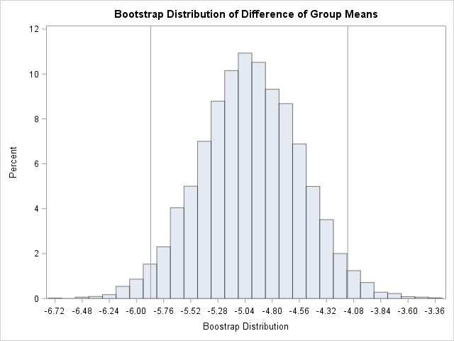
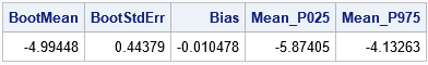
The results are shown. The bootstrap distribution appears to be normally distributed. This indicates that the bootstrap estimates will probably be similar to the classical parametric estimates. For this problem, the classical estimate of the standard error is 0.448 and a 95% confidence interval for the difference of means is [-5.87, -4.10]. In comparison, the bootstrap estimates are 0.444 and [-5.87, -4.13]. In spite of the skewness of the MPG_City variable for the “Sedan” group, the two-sample Satterthwaite t provides similar estimates regarding the accuracy of the point estimate for the difference of means.
The bootstrap statistics also are similar to the statistics that you can obtain by using the BOOTSTRAP statement in PROC TTEST in SAS/STAT 14.3.
In summary, you can use Base SAS and SAS/STAT procedures to compute a bootstrap analysis of a two-sample t test.
Although the “manual” bootstrap requires more programming effort than using the BOOTSTRAP statement in PROC TTEST, the example in this article generalizes to other statistics for which a built-in bootstrap option is not supported. This article also shows how to use PROC SURVEYSELECT to perform stratified sampling as part of a bootstrap analysis that involves sampling from multiple groups.
The post The bootstrap method in SAS: A t test example appeared first on The DO Loop.
| This post was kindly contributed by The DO Loop - go there to comment and to read the full post. |
↧
Balanced bootstrap resampling in SAS
| This post was kindly contributed by The DO Loop - go there to comment and to read the full post. |
This article shows how to implement balanced bootstrap sampling in SAS.
The basic bootstrap samples with replacement from the original data (N observations) to obtain B new samples. This is called “uniform” resampling because each observation has a uniform probability of 1/N of being selected at each step of the resampling process.
Within the union of the B bootstrap samples,
each observation has an expected value of appearing B times.
Balanced bootstrap resampling (Davison, Hinkley, and Schechtman, 1986) is an alternative process in which each observation appears exactly B times in the union of the B bootstrap samples of size N. This has some practical benefits for estimating certain inferential statistics such as the bias and quantiles of the sampling distribution (Hall, 1990).
It is easy to implement a balanced bootstrap resampling scheme: Concatenate B copies of the data, randomly permute the B*N observations, and then use the first N observations for the first bootstrap sample, the next B for the second sample, and so forth. (Other algorithms are also possible, as discussed by Gleason, 1988).
This article shows how to implement balanced bootstrap sampling in SAS.
Balanced bootstrap samples in SAS
To illustrate the idea, consider the following data set that has N=6 observations. Five observations are clustered near x=0 and the sixth is a large outlier (x=10). The sample skewness for these data is skew=2.316 because of the influence of the outlier.
data Sample(keep=x); input x @@; datalines; -1 -0.2 0 0.2 1 10 ; proc means data=Sample skewness; run; %let ObsStat = 2.3163714; |
You can use the bootstrap to approximate the sampling distribution for the skewness statistic for these data. I have previously shown how to use SAS to bootstrap the skewness statistic: Use PROC SURVEYSELECT to form bootstrap samples, use PROC MEANS with a BY statement to analyze the samples, and use PROC UNIVARIATE to analyze the bootstrap distribution of skewness values. In that previous article, PROC SURVEYSELECT is used to perform uniform sampling (sampling with replacement).
It is straightforward to modify the previous program to perform balanced bootstrap sampling. The following program is based on a SAS paper by Nils Penard at PhUSE 2012. It does the following:
- Use PROC SURVEYSEELCT to concatenate B copies of the input data.
- Use the DATA step to generate a uniform random number for each observation.
- Use PROC SORT to sort the data by the random values. After this step, the N*B observations are in random order.
- Generate a variable that indicates the bootstrap sample for each observation. Alternatively, reuse the REPLICATE variable from PROC SURVEYSELECT, as shown below.
/* balanced bootstrap computation */ proc surveyselect data=Sample out=DupData noprint reps=5000 /* duplicate data B times */ method=SRS samprate=1; /* sample w/o replacement */ run; data Permute; set DupData; call streaminit(12345); u = rand("uniform"); /* generate a uniform random number for each obs */ run; proc sort data=Permute; by u; run; /* sort in random order */ data BalancedBoot; merge DupData(drop=x) Permute(keep=x); /* reuse REPLICATE variable */ run; |
You can use the BalancedBoot data set to perform subsequent bootstrap analyses.
If you perform a bootstrap analysis, you obtain the following approximate bootstrap distribution for the skewness statistic. The observed statistic is indicated by a red vertical line. For reference, the mean of the bootstrap distribution is indicated by a gray vertical line. You can see that the sampling distribution for this tiny data set is highly nonnormal. Many bootstrap samples that contain the outlier (exactly one-sixth of the samples in a balanced bootstrap) will have a large skewness value.

To assure yourself that each of the original six observations appears exactly B times in the union of the bootstrap sample, you can run PROC FREQ, as follows:
proc freq data=BalancedBoot; /* OPTIONAL: Show that each obs appears B times */ tables x / nocum; run; |
Balanced bootstrap samples in SAS/IML
As shown in the article “Bootstrap estimates in SAS/IML,” you can perform bootstrap computations in the SAS/IML language.
For uniform sampling, the SAMPLE function samples with replacement from the original data. However, you can modify the sampling scheme to support balanced bootstrap resampling:
- Use the REPEAT function to duplicate the data B times.
- Use the SAMPLE function with the “WOR” option to sample without replacement. The resulting vector is a permutation of the B*N observations.
- Use the SHAPE function to reshape the permuted data into an N x B matrix for which each column is a bootstrap sample. This form is useful for implementing vectorized computations on the columns.
The following SAS/IML program modifies the program in the previous post to perform balanced bootstrap sampling:
/* balanced bootstrap computation in SAS/IML */ proc iml; use Sample; read all var "x"; close; call randseed(12345); /* Return a row vector of statistics, one for each column. */ start EvalStat(M); return skewness(M); /* <== put your computation here */ finish; Est = EvalStat(x); /* 1. observed statistic for data */ /* balanced bootstrap resampling */ B = 5000; /* B = number of bootstrap samples */ allX = repeat(x, B); /* replicate the data B times */ s = sample(allX, nrow(allX), "WOR"); /* 2. sample without replacement (=permute) */ s = shape(s, nrow(x), B); /* reshape to (N x B) */ /* use the balanced bootstrap samples in subsequent computations */ bStat = T( EvalStat(s) ); /* 3. compute the statistic for each bootstrap sample */ bootEst = mean(bStat); /* 4. summarize bootstrap distrib such as mean */ bias = Est - bootEst; /* Estimate of bias */ RBal = Est || BootEst || Bias; /* combine results for printing */ print RBal[format=8.4 c={"Obs" "BootEst" "Bias"}]; |

As shown in the previous histogram, the bias estimate (the difference between the observed statistic and the mean of the bootstrap distribution) is sizeable.
It is worth mentioning that the SAS-supplied
%BOOT macro performs balanced bootstrap sampling by default. To generate balanced bootstrap samples with the %BOOT macro, set the BALANCED=1 option, as follows:
%boot(data=Sample, samples=5000, balanced=1) /* or omit BALANCED= option */
If you want uniform (unbalanced) samples, call the macro as follows:
%boot(data=Sample, samples=5000, balanced=0).
In conclusion, it is easy to generate balanced bootstrap samples. Balanced sampling can improve the efficiency of certain bootstrap estimates and inferences. For details, see the previous references of Appendix II of Hall (1992).
The post Balanced bootstrap resampling in SAS appeared first on The DO Loop.
| This post was kindly contributed by The DO Loop - go there to comment and to read the full post. |
↧
↧
How to use the %BOOT and %BOOTCI macros in SAS
| This post was kindly contributed by The DO Loop - go there to comment and to read the full post. |
Since the late 1990s, SAS has supplied macros for basic bootstrap and jackknife analyses.
This article provides an example that shows how to use the %BOOT and %BOOTCI macros. The %BOOT macro generates a bootstrap distribution and computes basic statistics about the bootstrap distribution, including estimates of bias, standard error, and a confidence interval that is suitable when the sampling distribution is normally distributed.
Because bootstrap methods are often used when you do not want to assume a statistic is normally distributed, the %BOOTCI macro supports several additional confidence intervals, such as percentile-based and bias-adjusted intervals.
You can download the macros for free from the SAS Support website. The website includes additional examples, documentation, and a discussion of the capabilities of the macros.
The %BOOT macro uses simple uniform random sampling (with replacement) or balanced bootstrap sampling to generate the bootstrap samples.
It then calls a user-supplied %ANALYZE macro to compute the bootstrap distribution of your statistic.
How to install and use the %BOOT and %BOOTCI macros
To use the macros, do the following:
- Download the source file for the macros and save it in a directory that is accessible to SAS. For this example, I saved the source file to C:\Temp\jackboot.sas.
- Define a macro named %ANALYZE that computes the bootstrap statistic from a bootstrap sample. The next section provides an example.
- Call the %BOOT macro. The %BOOT macro creates three primary data sets:
- BootData is a data set view that contains B bootstrap samples of the data. For this example, I use B=5000.
- BootDist is a data set that contains the bootstrap distribution. It is created when the %BOOT macro internally calls the %ANALYZE macro on the BootData data set.
- BootStat is a data set that contains statistics about the bootstrap distribution. For example, the BootStat data set contains the mean and standard deviation of the bootstrap distribution, among other statistics.
- If you want confidence inervals, use the %BOOTCI macro to compute up to six different interval estimates. The %BOOTCI macro creates a data set named BootCI that contains the statistics that are used to construct the confidence interval. (You can also generate multiple interval estimates by using the %ALLCI macro.)
An example of calling the %BOOT macro
This section shows how to call the %BOOT macro. The example was previously analyzed in an article that shows how to compute a bootstrap percentile confidence interval in SAS. The statistic of interest is the skewness of the SepalWidth variable for 50 iris flowers of the species Iris virginica. The following SAS statements define the sample data and compute the skewness statistic on the original data.
%include "C:\Temp\jackboot.sas"; /* define the %BOOT and %BOOTCI macros */ data sample(keep=x); /* data are sepal widths for 50 Iris virginica flowers */ set Sashelp.Iris(where=(Species="Virginica") rename=(SepalWidth=x)); run; /* compute value of the statistic on original data: Skewness = 0.366 */ title 'Skewness for Petal Widths (Iris virginica)'; proc means data=sample nolabels skewness; var x; output out=SkewOut skew=Skewness; /* three output variables: _type_ _freq_ and Skewness */ run; |
The skewness statistic (not shown) is 0.366. The call to PROC MEANS is not necessary, but it shows how to create an output data set (SkewOut) that contains the Skewness statistic. By default, the %BOOT macro will analyze all numeric variables in the output data set, so the next step defines the %ANALYZE macro and uses the DROP= data set option to omit some unimportant variables that PROC MEANS automatically generates.
When you define the %ANALYZE macro, be sure to use the NOPRINT option or otherwise suppress ODS output during the bootstrap process. Include the %BYSTMT macro, which will tell the %BOOT macro to use a BY statement to efficiently implement the bootstrap analysis. The %ANALYZE macro is basically the same as the previous call to PROC MEANS, except for the addition of the NOPRINT, %BYSTMT, and DROP= options:
%macro analyze(data=,out=); proc means noprint data=&data; %bystmt; var x; output out=&out(drop=_type_ _freq_) skew=Skewness; run; %mend; |
Although the DROP= statement is not essential, it reduces the size of the data that are read and written during the bootstrap analysis. Do NOT use a KEEP= statement in the %ANALYZE macro because the %BOOT macro will generate several other variables (called _SAMPLE_ and _OBS_) as part of the resampling process.
You can now use the %BOOT macro to generate bootstrap samples and compute basic descriptive statistics about the bootstrap distribution:
/* creates GootData, BootDist, and BootStat data sets */ title2 'Bootstrap Analysis of Skewness'; %boot(data=sample, /* data set that contains the original data */ samples=5000, /* number of bootstrap samples */ random=12345, /* random number seed for resampling */ chart=0, /* do not display the old PROC CHART histograms */ stat=Skewness, /* list of output variables to analyze (default=_NUMERIC_) */ alpha=0.05, /* significance level for CI (default=0.05) */ print=1); /* print descriptive stats (default=1)*/ proc print data=bootstat noobs; /* or use LABEL option to get labels as column headers */ id method n; var value bootmean bias stderr biasco alcl aucl; run; |

I recommend that you specify the first four options. The last three options are shown in case you want to override their default values. Although the %BOOT macro prints a table of descriptive statistics, the table contains 14 columns and is very wide. To shorten the output, I used PROC PRINT to display the most important results. The table shows the estimate of the skewness statistic on the original data (VALUE), the mean of the bootstrap distribution (BOOTMEAN), the estimate for the standard error of the statistic (STDERR), and lower and upper confidence limits (ALCL and AUCL) for an approximate confidence interval under the assumption that the statistic is normally distributed. (The limits are b ± z1-α * stderr, where z1-α is the (1 – α)th normal quantile and b = value – bias is a bias-corrected estimate.)
The data for the bootstrap distribution is in the BootDist data set, so you can use PROC SGPLOT to display a histogram of the bootstrap statistics. I like to assign some of the descriptive statistics into macro variables so that I can display them on the histogram, as follows:
/* OPTIONAL: Store bootstrap statistic in a macro variable */ proc sql noprint; select value, alcl, aucl into :Stat, :LowerCL, :UpperCL from BootStat; quit; proc sgplot data=BootDist; /* <== this data set contains the bootstrap distribution */ histogram Skewness; refline &Stat / axis=x lineattrs=(color=red); refline &LowerCL &UpperCL / axis=x; run; |
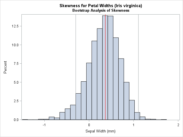
An example of calling the %BOOTCI macro
The %BOOTCI macro enables you to compute several confidence intervals (CIs) for the statistic that you are bootstrapping. The following statements display a percentile-based CI and a bias-adjusted and corrected CI.
title2 'Percentile-Based Confidence Interval'; %bootci(PCTL); /* creates BootCI data set for Pctl CI */ |
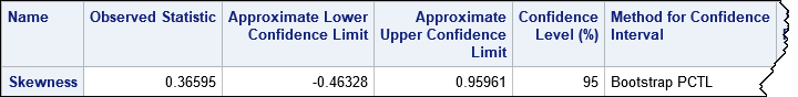
The percentile-based CI is about the same width as the normal-based CI, but it is shifted to the left. The default output from the %BOOTCI macro is very wide, so sometimes I prefer to use the PRINT=0 option to suppress the output. The estimates are written to a data set named BootCI, so it is easy to use PROC PRINT to display only the statistics that you want to see, as shown in the following call that computes a bias-corrected and adjusted interval estimate:
title2 'Bias-Adjusted and Corrected Bootstrap Confidence Interval'; %bootci(BCa, print=0); /* creates BootCI data set for BCa CI */ proc print data=BootCI noobs label; id method n; var value alcl aucl; run; |
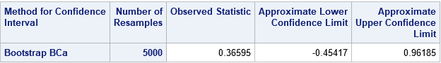
Notice that each call to the %BOOTCI macro creates a data set named BootCI. In particular, the second call overwrites the data set that was created by the first call. If you want to compare the estimates, be sure to make a copy of the first BootCI data set before you overwrite it.
The %ALLCI macro
If you want to compare multiple CIs, you can use the %ALLCI macro, which computes multiple definitions of the CIs and concatenates them into a data set named AllCI, as shown by the following:
title2 'Comparison of Bootstrap Confidence Intervals'; %allci(print=0); proc print data=AllCI(drop=_LABEL_) noobs label; id method n; var value alcl aucl; run; |
The output (not shown) contains interval estimates for five bootstrap CIs and a jackknife CI.
Be aware the when you run the %ALLCI macro you will see several warnings in the SAS log, such as the following:
WARNING: Variable _lo was not found on DATA file.
WARNING: Variable bootmean was not found on BASE file. The variable will
         not be added to the BASE file.
|
These warnings are coming from PROC APPEND and can be ignored.
To suppress these warnings, you can edit the jackboot.sas file, search for the word ‘force’ on the PROC APPEND statements, and add the NOWARN option to those PROC APPEND statements. For example:
proc append data=bootci&keep base=ALLCI force nowarn; run;
Pros and cons of using the %BOOT macro
The %BOOT, %BOOTCI, and %ALLCI macros can be a time-saver when you want to perform a basic bootstrap in SAS. However, in my opinion, they are not a substitute for understanding how to implement a bootstrap computation manually in SAS. Here are a few advantages and disadvantages of the macros:
- Advantage: The macros encapsulate the tedious steps of the bootstrap analysis.
- Advantage: The macros generate SAS data sets that you can use for additional analyses or for graphing the results.
- Advantage: The macros handle the most common sampling schemes such as simple uniform sampling (with replacement), balanced bootstrap sampling, and residual sampling in regression models.
- Advantage: The %BOOTCI macro supports many popular confidence intervals for parameters.
- Disadvantage: The macros do not provide the same flexibility as writing your own analysis. For example, the macros do not support the stratified resampling scheme that is used for a bootstrap analysis of the difference of means in a t test.
- Disadvantage: There are only a few examples of using the macros. When I first used them, I made several mistakes and had to look at the underlying source code to understand what the macros were doing.
Summary
The %BOOT and %BOOTCI macros provide a convenient way to perform simple bootstrap analyses in SAS.
The macros support several common resampling schemes and estimates for confidence intervals. Although the macros are not a replacement for understanding how to program a general, efficient, bootstrap analysis, they can be a useful tool for data analysts who want compact code to create a bootstrap analysis in SAS.
The post How to use the %BOOT and %BOOTCI macros in SAS appeared first on The DO Loop.
| This post was kindly contributed by The DO Loop - go there to comment and to read the full post. |
↧
Bootstrap regression estimates: Case resampling
| This post was kindly contributed by The DO Loop - go there to comment and to read the full post. |
If you want to bootstrap the parameters in a statistical regression model, you have two primary choices.
The first is case resampling, which is also called resampling observations or resampling pairs. In case resampling, you create the bootstrap sample by randomly selecting observations (with replacement) from the original data.
The second choice is called resampling residuals. In this method, you fit a model to the original data to obtain predicted values and residuals. You create the bootstrap sample by using the original explanatory variables but construct a new response value by adding a random residual to the predicted value.
This article shows an example of case resampling in SAS.
A future article shows an example of resampling residuals.
Case resampling for bootstrapping a regression analysis
If you have some experience with bootstrapping univariate statistics, case resampling will look familiar.
The main ideas behind bootstrapping are explained in the article
“Compute a bootstrap confidence interval in SAS,” which discusses the following steps of the bootstrap method:
- Compute the statistic of interest for the original data
- Resample B times from the data to form B bootstrap samples.
- Compute the statistic on each bootstrap sample. This creates the bootstrap distribution, which approximates the sampling distribution of the statistic.
- Use the approximate sampling distribution to obtain bootstrap estimates such as standard errors, confidence intervals, and evidence for or against the null hypothesis.
To demonstrate case resampling, consider the sampling distribution of the parameter estimates (the regression coefficients) in an ordinary least squares (OLS) regression.
The sampling distribution gives insight into the variation of the estimates and how the estimates are correlated.
In a case-resampling analysis, each bootstrap sample will contain randomly chosen observations from the original data. You fit the same regression model to each sample to obtain the bootstrap estimates. You can then analyze the distribution of the bootstrap estimates.
For the statistics in this article, you can compare the bootstrap estimates with estimates of standard errors and confidence intervals (CIs) that are produced by PROC REG in SAS. The procedure constructs the statistics based on several assumptions about the distribution of the errors in the OLS model.
In contrast, bootstrap estimates are nonparametric and rely on fewer assumptions. Thus bootstrapping is useful when you are not sure whether the OLS assumptions hold for your data, or when you want to obtain confidence intervals for statistics (like the R-squared and RMSE) that have complicated or unknown sampling distributions.
The statistic of interest for the original data
This example analyzes the Sashelp.Class data set, which contains data about the weights and heights of 19 students. The response variable is the Weight variable, which you can regress onto the Height variable. The regression produces two parameter estimates (Intercept and Height), standard errors, and an estimate of the “covariance of the betas.”
For clarity, I rename the response variable to Y and the explanatory variable to X so that each variable’s role is obvious.
/* regression bootstrap: case resampling */ data sample(keep=x y); set Sashelp.Class(rename=(Weight=Y Height=X)); /* rename to make roles easier to understand */ run; /* 1. compute the statistics on the original data */ proc reg data=Sample plots=none; model Y = X / CLB covb; /* original estimates */ run; quit; |
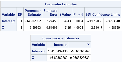
The “Parameter Estimates” table includes point estimates, standard errors, and confidence intervals for the regression coefficients. The “Covariance of Estimates” table shows that the estimates are negatively correlated.
Resample from the data
The following call to PROC SURVEYSELECT creates 5,000 bootstrap samples by sampling with replacement from the data:
title "Bootstrap Distribution of Regression Estimates"; title2 "Case Resampling"; %let NumSamples = 5000; /* number of bootstrap resamples */ %let IntEst = -143.02692; /* original estimates for later visualization */ %let XEst = 3.89903; /* 2. Generate many bootstrap samples by using PROC SURVEYSELECT */ proc surveyselect data=sample NOPRINT seed=1 out=BootCases(rename=(Replicate=SampleID)) method=urs /* resample with replacement */ samprate=1 /* each bootstrap sample has N observations */ /* OUTHITS use OUTHITS option to suppress the frequency var */ reps=&NumSamples; /* generate NumSamples bootstrap resamples */ run; |
The output from the SURVEYSELECT procedure is a large data set (BootCases) that contains all bootstrap samples. The SampleID variable indicates which observations belong to each sample. The NumberHits variable gives the frequency for which each of the original observations is selected. That variable should be used as a FREQ variable when analyzing the bootstrap samples. (If your procedure does not have support for a frequency variable, use the OUTHITS option on the PROC SURVEYSELECT statement to obtain an “expanded” version of the bootstrap samples.)
Compute the bootstrap distribution
The BootCases data set contains 5,000 bootstrap samples. You can perform 5,000 regression analyses efficiently by using a BY-group analysis. You can use the BY statement in PROC REG. Be sure to use the NOPRINT option to suppress the output to the screen and use the OUTEST= option to create an output data set that contains 5,000 parameter estimates, one for each bootstrap sample.
/* 3. Compute the statistic for each bootstrap sample */ proc reg data=BootCases outest=PEBoot noprint; by SampleID; freq NumberHits; model Y = X; run;quit; |
Analyze the bootstrap distribution
The PEBoot data set contains 5,000 parameter estimates. To visualize the bootstrap distribution, you can create a scatter plot. The following call to PROC SGPLOT overlays reference lines that intersect at the parameter estimates for the original data.
/* 4. Visualize bootstrap distribution */ proc sgplot data=PEBoot; label Intercept = "Estimate of Intercept" X = "Estimate of Coefficient of X"; scatter x=Intercept y=X / markerattrs=(Symbol=CircleFilled) transparency=0.7; /* Optional: draw reference lines at estimates for original data */ refline &IntEst / axis=x lineattrs=(color=blue); refline &XEst / axis=y lineattrs=(color=blue); xaxis grid; yaxis grid; run; |
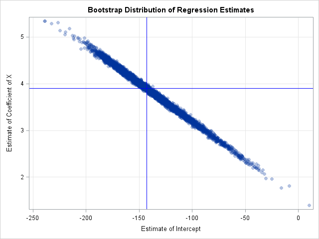
The scatter plot shows that the estimates are negatively correlated, which was previously shown by the output from the COVB option on the original data. You can call PROC CORR on the bootstrap samples to obtain a bootstrap estimate of the covariance of the betas:
proc corr data=PEBoot cov vardef=N; var Intercept X; run; |
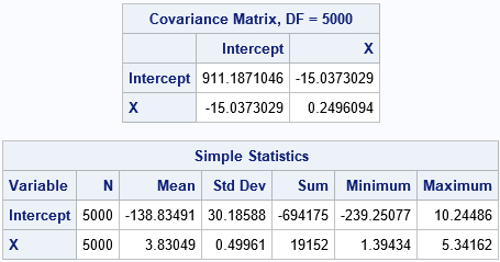
The covariance matrix for the bootstrap estimates is close to the COVB matrix from PROC REG. The “Simple Statistics” table shows other bootstrap estimates. The Mean column shows the average of the bootstrap estimates; the difference between the original parameter estimates and the bootstrap average is an estimate of bias.
The StdDev column estimates the standard errors of the regression estimates.
You can also use the 0.025 and 0.975 quantiles of the bootstrap estimates to construct a 95% confidence interval for the parameters. There are many ways to get the percentiles in SAS. the following statements call PROC STDIZE and print the confidence intervals for the Intercept and X variables:
proc stdize data=PEBoot vardef=N pctlpts=2.5 97.5 PctlMtd=ORD_STAT outstat=Pctls; var Intercept X; run; proc report data=Pctls nowd; where _type_ =: 'P'; label _type_ = 'Confidence Limit'; columns ('Bootstrap Confidence Intervals (B=5000)' _ALL_); run; |
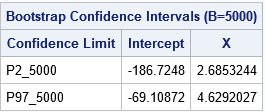
The bootstrap estimates of the confidence intervals are shorter than the Wald confidence intervals from PROC REG that assume normality of errors.
Summary
In summary, there are two primary ways to perform bootstrapping for parameters in a regression model. This article generates bootstrap samples by using
“case resampling” in which observations are randomly selected (with replacement). The bootstrap process enables you to estimate the standard errors, confidence intervals, and covariance (or correlation) of the estimates. You can also use the %BOOT macro to carry out this kind of bootstrap analysis.
Case resampling is a good choice when you are modeling observational data in which the explanatory variables are observed randomly from a population. Although OLS regression treats the explanatory variable (such as Height) as a fixed effect,
if you were to go into a different school and randomly select 19 students from the same grade, you would obtain a different set of heights. In that sense, the data (X and Y) can be thought of as random values from a larger population.
If you are analyzing data from a designed experiment in which the explanatory variables have a small number of specified values, you can use residual resampling, which is discussed in the next blog post.
The post Bootstrap regression estimates: Case resampling appeared first on The DO Loop.
| This post was kindly contributed by The DO Loop - go there to comment and to read the full post. |
↧
Bootstrap regression estimates: Residual resampling
| This post was kindly contributed by The DO Loop - go there to comment and to read the full post. |
If you want to bootstrap the parameters in a statistical regression model, you have two primary choices.
The first, case resampling, is discussed in a previous article. This article describes the second choice, which is resampling residuals (also called model-based resampling). This article shows how to implement residual resampling in Base SAS and in the SAS/IML matrix language.
Residual resampling assumes that the model is correctly specified and that the error terms in the model are identically distributed and independent. However, the errors do not need to be normally distributed. Before you run a residual-resampling bootstrap, you should use regression diagnostic plots to check whether there is an indication of heteroskedasticity or autocorrelation in the residuals. If so, do not use this bootstrap method.
Although residual resampling is primarily used for designed experiments, this article uses the same data set as in the previous article: the weights (Y) and heights (X) of 19 students. Therefore, you can compare the results of the two bootstrap methods. As in the previous article, this article uses the bootstrap to examine the sampling distribution and variance of the parameter estimates (the regression coefficients).
Bootstrap residuals
The following steps show how to bootstrap residuals in a regression analysis:
- Fit a regression model that regresses the original response, Y, onto the explanatory variables, X. Save the predicted values (YPred) and the residual values (R).
- A bootstrap sample consists of forming a new response vector as Yi, Boot = Yi, Pred + Rrand, where
Yi, Pred is the i_th predicted value and Rrand is chosen randomly (with replacement) from the residuals in Step 1. Create B samples, where B is a large number. - For each bootstrap sample, fit a regression model that regresses YBoot onto X.
- The bootstrap distribution is the union of all the statistics that you computed in Step 3. Analyze the bootstrap distribution to estimate standard errors and confidence intervals for the parameters.
Step 1: Fit a model, save predicted and residual values
To demonstrate residual resampling, I will use procedures in Base SAS and SAS/STAT. (A SAS/IML solution is presented at the end of this article.)
The following statements create the data and rename the response variable (Weight) and the explanatory variable (X) so that their roles are clear. Step 1 of the residual bootstrap is to fit a model and save the predicted and residual values:
data sample(keep=x y); set Sashelp.Class(rename=(Weight=Y Height=X)); run; /* 1. compute value of the statistic on original data */ proc reg data=Sample plots=none; model Y = X / CLB covb; output out=RegOut predicted=Pred residual=Resid; run; quit; %let IntEst = -143.02692; /* set some macro variables for later use */ %let XEst = 3.89903; %let nObs = 19; |
Step 2: Form the bootstrap resamples
The second step is to randomly draw residuals and use them to generate new response vectors from the predicted values of the fitted model. There are several ways to do this. If you have SAS 9.4m5 (SAS/STAT 14.3), you can use PROC SURVEYSELECT to select and output the residuals in a random order. An alternative method that uses the SAS DATA step is shown below. The program reads the residuals into an array. For each original observation, it adds a random residual to the predicted response. It does this B times, where B = 5,000. It then sorts the data by the SampleID variable so that the B bootstrap samples are ready to be analyzed.
%let NumSamples = 5000; /* B = number of bootstrap resamples */ /* SAS macro: chooses random integer in [min, max]. See https://blogs.sas.com/content/iml/2015/10/05/random-integers-sas.html */ %macro RandBetween(min, max); (&min + floor((1+&max-&min)*rand("uniform"))) %mend; /* 2. For each obs, add random residual to predicted values to create a random response. Do this B times to create all bootstrap samples. */ data BootResiduals; array _residual[&nObs] _temporary_; /* array to hold residuals */ do i=1 to &nObs; /* read data; put rasiduals in array */ set RegOut point=i; _residual[i] = Resid; end; call streaminit(12345); /* set random number seed */ set RegOut; /* for each observations in data */ ObsID = _N_; /* optional: keep track of obs position */ do SampleId = 1 to &NumSamples; /* for each bootstrap sample */ k = %RandBetween(1, &nObs); /* choose a random residual */ YBoot = Pred + _residual[k]; /* add it to predicted value to create new response */ output; end; drop k; run; /* prepare for BY group analysis: sort by SampleID */ proc sort data=BootResiduals; by SampleID ObsID; /* sorting by ObsID is optional */ run; |
Step 3: Analyze the bootstrap resamples
The previous step created a SAS data set (BootResiduals) that contains B = 5,000 bootstrap samples. The unique values of the SampleID variable indicate which observations belong to which sample. You can use a BY-group analysis to efficiently analyze all samples in a single call to PROC REG, as follows:
/* 3. analyze all bootstrap samples; save param estimates in data set */ proc reg data=BootResiduals noprint outest=PEBootResid; by SampleID; model YBoot = X; run;quit; /* take a peek at the first few bootstrap estimates */ proc print data=PEBootResid(obs=5); var SampleID Intercept X; run; |
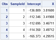
The result of the analysis is a data set (PEBootResid) that contains 5,000 rows. The i_th row contains the parameter estimates for the i_th bootstrap sample. Thus, the Intercept and X columns contain the bootstrap distribution of the parameter estimates, which approximates the sampling distribution of those statistics.
Step 4: Analyze the bootstrap distribution
The previous article includes SAS code that estimates the standard errors and covariance of the parameter estimates. It also provides SAS code for a bootstrap confidence interval for the parameters. I will not repeat those computations here. The following call to PROC SGPLOT displays a scatter plot of the bootstrap distribution of the estimates. You can see from the plot that the estimates are negatively correlated:
/* 4. Visualize and analyze the bootstrap distribution */ title "Parameter Estimates for &NumSamples Bootstrap Samples"; title2 "Residual Resampling"; proc sgplot data=PEBootResid; label Intercept = "Estimate of Intercept" X = "Estimate of Coefficient of X"; scatter x=Intercept y=X / markerattrs=(Symbol=CircleFilled) transparency=0.7; /* Optional: draw reference lines at estimates for original data */ refline &IntEst / axis=x lineattrs=(color=blue); refline &XEst / axis=y lineattrs=(color=blue); xaxis grid; yaxis grid; run; |
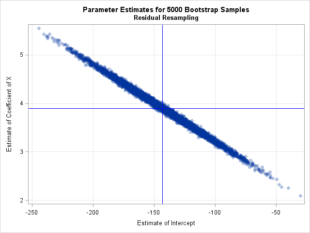
Bootstrap residuals in SAS/IML
For standard regression analyses, the previous sections show how to bootstrap residuals in a regression analysis in SAS. If you are doing a nonstandard analysis, however, you might need to perform a bootstrap analysis in the SAS/IML language. I’ve previously shown how to perform a bootstrap analysis (using case resampling) in SAS/IML. I’ve also shown how to use the SWEEP operator in SAS/IML to run thousands of regressions in a single statement. You can combine these ideas, along with an easy way to resample data (with replacement) in SAS/IML, to write a short SAS/IML program that resamples residuals, fits the samples, and plots the bootstrap estimates:
proc iml; use RegOut; read all var {Pred X Resid}; close; /* read data */ design = j(nrow(X), 1, 1) || X; /* design matrix for explanatory variables */ /* resample residuals with replacement; form bootstrap responses */ call randseed(12345); R = sample(Resid, &NumSamples//nrow(Resid)); /* NxB matrix; each col is random residual */ YBoot = Pred + R; /* 2. NxB matrix; each col is Y_pred + resid */ M = design || YBoot; /* add intercept and X columns */ ncol = ncol(M); MpM = M`*M; /* (B+2) x (B+2) crossproduct matrix */ free R YBoot M; /* free memory */ /* Use SWEEP function to run thousands of regressions in a single call */ S = sweep(MpM, {1 2}); /* 3. sweep in intercept and X for each Y_i */ ParamEst = S[{1 2}, 3:ncol]; /* estimates for models Y_i = X */ /* 4. perform bootstrap analyses by analyzing ParamEst */ call scatter(ParamEst[1,], ParamEst[2,]) grid={x y} label={"Intercept" "X"} other="refline &IntEst /axis=x; refline &XEst /axis=y;"; |
The graph is similar to the previous scatter plot and is not shown. It is remarkable how concise the SAS/IML language can be, especially compared to the procedure-based approach in Base SAS. On the other hand, the SAS/IML program uses a crossproduct matrix (MpM) that contains approximately B2 elements. If you want to analyze, say, B = 100,000 bootstrap samples, you would need to restructure the program. For example, you could analyze 10,000 samples at a time and accumulate the bootstrap estimates.
Further thoughts and summary
The %BOOT macro also supports resampling residuals in a regression context. The documentation for the %BOOT macro contains an example.
No matter how you choose to bootstrap residuals, remember that the process
assumes that the model is correct and that the error terms in the model are identically distributed and independent.
Use caution if the response variable has a physical meaning, such as a physical dimension that must be positive (length, weight, …). When you create a new response as the sum of a predicted value and a random residual, you might obtain an unrealistic result, especially if the data contain an extreme outlier. If your resamples contain a negative length or a child whose height is two meters, you might reconsider whether resampling residuals is appropriate for your data and model.
When it is appropriate, the process of resampling residuals offers a way to use the bootstrap to investigate the variance of many parameters that arise in regression. It is especially useful for data from experiments in which the explanatory variables have values that are fixed by the design.
The post Bootstrap regression estimates: Residual resampling appeared first on The DO Loop.
| This post was kindly contributed by The DO Loop - go there to comment and to read the full post. |
↧