Bootstrap estimates in SAS/IML

I previously wrote about how to compute a bootstrap confidence interval in Base SAS. As a reminder, the bootstrap method consists of the following steps:

1. Compute the statistic of interest for the original data
2. Resample B times from the data to form B bootstrap samples. B is usually a large number, such as B = 5000.
3. Compute the statistic on each bootstrap sample. This creates the bootstrap distribution, which approximates the sampling distribution of the statistic.
4. Use the bootstrap distribution to obtain bootstrap estimates such as standard errors and confidence intervals.

In my book Simulating Data with SAS, I describe efficient ways to bootstrap in the SAS/IML matrix language. Whereas the Base SAS implementation of the bootstrap requires calls to four or five procedure, the SAS/IML implementation requires only a few function calls. This article shows how to compute a bootstrap confidence interval from percentiles of the bootstrap distribution for univariate data. How to bootstrap multivariate data is discussed on p. 189 of Simulating Data with SAS.

Skewness of univariate data

Let’s use the bootstrap to find a 95% confidence interval for the skewness statistic. The data are the petal widths of a sample of 50 randomly selected flowers of the species Iris setosa. The measurements (in mm) are contained in the data set Sashelp.Iris.
So that you can easily generalize the code to other data, the following statements create a data set called SAMPLE and the rename the variable to analyze to ‘X’. If you do the same with your data, you should be able to reuse the program by modifying only a few statements.

The following DATA step renames the data set and the analysis variable. A call to PROC UNIVARIATE graphs the data and provides a point estimate of the skewness:

data sample;
   set sashelp.Iris;     /* <== load your data here */
   where species = "Setosa";
   rename PetalWidth=x;  /* <== rename the analyzes variable to 'x' */
run;
 
proc univariate data=sample;
   var x;
   histogram x;
   inset N Skewness (6.3) / position=NE;
run;

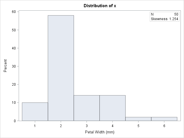
The petal widths have a highly skewed distribution, with a skewness estimate of 1.25.

A bootstrap analysis in SAS/IML

Running a bootstrap analysis in SAS/IML requires only a few lines to compute the confidence interval, but to help you generalize the problem to statistics other than the skewness, I wrote a function called EvalStat. The input argument is a matrix where each column is a bootstrap sample. The function returns a row vector of statistics, one for each column. (For the skewness statistic, the EvalStat function is a one-liner.) The EvalStat function is called twice: once on the original column vector of data and again on a matrix that contains bootstrap samples in each column. You can create the matrix by calling the SAMPLE function in SAS/IML, as follows:

/* Basic bootstrap percentile CI. The following program is based on 
   Chapter 15 of Wicklin (2013) Simulating Data with SAS, pp 288-289. 
*/
proc iml;
/* Function to evaluate a statistic for each column of a matrix.
   Return a row vector of statistics, one for each column. */
start EvalStat(M); 
   return skewness(M);               /* <== put your computation here */
finish;
 
alpha = 0.05;
B = 5000;                            /* B = number of bootstrap samples */
use sample; read all var "x"; close; /* read univariate data into x */
 
call randseed(1234567);
Est = EvalStat(x);                   /* 1. compute observed statistic */
s = sample(x, B // nrow(x));         /* 2. generate many bootstrap samples (N x B matrix) */
bStat = T( EvalStat(s) );            /* 3. compute the statistic for each bootstrap sample */
bootEst = mean(bStat);               /* 4. summarize bootstrap distrib such as mean, */
SE = std(bStat);                             /* standard deviation,                  */
call qntl(CI, bStat, alpha/2 || 1-alpha/2);  /* and 95% bootstrap percentile CI      */
 
R = Est || BootEst || SE || CI`;     /* combine results for printing */
print R[format=8.4 L="95% Bootstrap Pctl CI"  
        c={"Obs" "BootEst" "StdErr" "LowerCL" "UpperCL"}];

The SAS/IML program for the bootstrap is very compact. It is important to keep track of the dimensions of each variable. The EST, BOOTEST, and SE variables are scalars. The S variable is a B x N matrix, where N is the sample size. The BSTAT variable is a column vector with N elements. The CI variable is a two-element column vector.

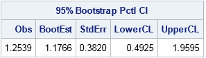
The output summarizes the bootstrap analysis. The estimate for the skewness of the observed data is 1.25. The bootstrap distribution (the skewness of the bootstrap samples) enables you to estimate three common quantities:

• The bootstrap estimate of the skewness is 1.18. This value is computed as the mean of the bootstrap distribution.
• The bootstrap estimate of the standard error of the skewness is 0.38. This value is computed as the standard deviation of the bootstrap distribution.
• The bootstrap percentile 95% confidence interval is computed as the central 95% of the bootstrap estimates, which is the interval
  [0.49, 1.96].

It is important to realize that these estimate will vary slightly if you use different random-number seeds or a different number of bootstrap iterations (B).

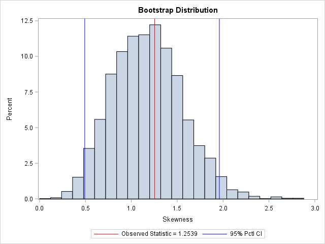
You can visualize the bootstrap distribution by drawing a histogram of the bootstrap estimates. You can overlay the original estimate (or the bootstrap estimate) and the endpoints of the confidence interval, as shown below.

In summary, you can implement the bootstrap method in the SAS/IML language very compactly.
You can use the bootstrap distribution to estimate the
parameter and standard error.
The bootstrap percentile method, which is based on quantiles of the bootstrap distribution, is a simple way to obtain a confidence interval for a parameter.

You can download the full SAS program that implements this analysis.

The post Bootstrap estimates in SAS/IML appeared first on The DO Loop.